Encoding Statistical Independence, Statically

Applicative functors are useful for encoding context-free effects. This typically gets put to work around things like parsing or validation, but if you have a statistical bent then an applicative structure will be familiar to you as an encoder of independence.

In this article I’ll give a whirlwind tour of probability monads and algebraic freeness, and demonstrate that applicative functors can be used to represent independence between probability distributions in a way that can be verified statically.

I’ll use the following preamble for the code in the rest of this article. You’ll need the free and mwc-probability libraries if you’re following along at home:

{-# LANGUAGE DeriveFunctor #-}
{-# LANGUAGE LambdaCase #-}

import Control.Applicative
import Control.Applicative.Free
import Control.Monad
import Control.Monad.Free
import Control.Monad.Primitive
import System.Random.MWC.Probability (Prob)
import qualified System.Random.MWC.Probability as MWC

Probability Distributions and Algebraic Freeness

Many functional programmers (though fewer statisticians) know that probability has a monadic structure. This can be expressed in multiple ways; the discrete probability distribution type found in the PFP framework, the sampling function representation used in the lambda-naught paper (and implemented here, for example), and even an obscure measure-based representation first described by Ramsey and Pfeffer, which doesn’t have a ton of practical use.

The monadic structure allows one to sequence distributions together. That is: if some distribution ‘foo’ has a parameter which itself has the probability distribution ‘bar’ attached to it, the compound distribution can be expressed by the monadic expression ‘bar »= foo’.

At a larger scale, monadic programs like this correspond exactly to what you’d typically see in a run-of-the-mill visualization of a probabilistic model:

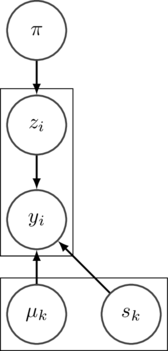
In this classical kind of visualization the nodes represent probability distributions and the arrows describe the dependence structure. Translating it to a monadic program is mechanical: the nodes become monadic expressions and the arrows become binds. You’ll see a simple example in this article shortly.

The monadic structure of probability implies that it also has a functorial structure. Mapping a function over some probability distrubution will transform its support while leaving its probability density structure invariant in some sense. If the function ‘uniform’ defines a uniform probability distribution over the interval (0, 1), then the function ‘fmap (+ 1) uniform’ will define a probability distribution over the interval (1, 2).

I’ll come back to probability shortly, but the point is that probability distributions have a clear and well-defined algebraic structure in terms of things like functors and monads.

Recently free objects have become fashionable in functional programming. I won’t talk about it in detail here, but algebraic ‘freeness’ corresponds to a certain preservation of structure, and exploiting this kind of preserved structure is a useful technique for writing and interpreting programs.

Gabriel Gonzalez famously wrote about freeness in an oft-cited article about free monads, John De Goes wrote a compelling piece on the topic in the excellent A Modern Architecture for Functional Programming, and just today I noticed that Chris Stucchio had published an article on using Free Boolean Algebras for implementing a kind of constraint DSL. The last article included the following quote, which IMO sums up much of the raison d’être to exploit freeness in your day-to-day work:

.. if you find yourself re-implementing the same algebraic structure over and over, it might be worth asking yourself if a free version of that algebraic structure exists. If so, you might save yourself a lot of work by using that.

If a free version of some structure exists, then it embodies the ‘essence’ of that structure, and you can encode specific instances of it by just layering the required functionality over the free object itself.

A Type for Probabilistic Models

Back to probability. Since probability distributions are monads, we can use a free monad to encode them in a structure-preserving way. Here I’ll define a simple probability base functor for which each constructor is a particular ‘named’ probability distribution:

data ProbF r =
    BetaF Double Double (Double -> r)
  | BernoulliF Double (Bool -> r)
  deriving Functor

type Model = Free ProbF

Here we’ll only work with two simple named distributions - the beta and the Bernoulli - but the sky is the limit.

The ‘Model’ type wraps up this probability base functor in the free monad, ‘Free’. In this sense a ‘Model’ can be viewed as a program parameterized by the underlying probabilistic instruction set defined by ‘ProbF’ (a technique I described recently).

Expressions with the type ‘Model’ are terms in an embedded language. We can create some user-friendly ones for our beta-bernoulli language like so:

beta :: Double -> Double -> Model Double
beta a b = liftF (BetaF a b id)

bernoulli :: Double -> Model Bool
bernoulli p = liftF (BernoulliF p id)

Those primitive terms can then be used to construct expressions.

The beta and Bernoulli distributions enjoy an algebraic property called conjugacy that ensures (amongst other things) that the compound distribution formed by combining the two of them is analytically tractable. Here’s a parameterized coin constructed by doing just that:

coin :: Double -> Double -> Model Bool
coin a b = beta a b >>= bernoulli

By tweaking the parameters ‘a’ and ‘b’ we can bias the coin in particular ways, making it more or less likely to observe a head when it’s inspected.

A simple evaluator for the language goes like this:

eval :: PrimMonad m => Model a -> Prob m a
eval = iterM $ \case
  BetaF a b k    -> MWC.beta a b >>= k
  BernoulliF p k -> MWC.bernoulli p >>= k

‘iterM’ is a monadic, catamorphism-like recursion scheme that can be used to succinctly consume a ‘Model’. Here I’m using it to propagate uncertainty through the model by sampling from it ancestrally in a top-down manner. The ‘MWC.beta’ and ‘MWC.bernoulli’ functions are sampling functions from the mwc-probability library, and the resulting type ‘Prob m a’ is a simple probability monad type based on sampling functions.

To actually sample from the resulting ‘Prob’ type we can use the system’s PRNG for randomness. Here are some simple coin tosses with various biases as an example; you can mentally substitute ‘Head’ for ‘True’ if you’d like:

> gen <- MWC.createSystemRandom
> replicateM 10 $ MWC.sample (eval (coin 1 1)) gen
[False,True,False,False,False,False,False,True,False,False]
> replicateM 10 $ MWC.sample (eval (coin 1 8)) gen
[False,False,False,False,False,False,False,False,False,False]
> replicateM 10 $ MWC.sample (eval (coin 8 1)) gen
[True,True,True,False,True,True,True,True,True,True]

As a side note: encoding probability distributions in this way means that the other ‘forms’ of probability monad described previously happen to fall out naturally in the form of specific interpreters over the free monad itself. A measure-based probability monad could be achieved by using a different ‘eval’ function; the important monadic structure is already preserved ‘for free’:

measureEval :: Model a -> Measure a
measureEval = iterM $ \case
  BetaF a b k    -> Measurable.beta a b >>= k
  BernoulliF p k -> Measurable.bernoulli p >>= k

Independence and Applicativeness

So that’s all cool stuff. But in some cases the monadic structure is more than what we actually require. Consider flipping two coins and then returning them in a pair, for example:

flips :: Model (Bool, Bool)
flips = do
  c0 <- coin 1 8
  c1 <- coin 8 1
  return (c0, c1)

These coins are independent - they don’t affect each other whatsoever and enjoy the probabilistic/statistical property that formalizes that relationship. But the monadic program above doesn’t actually capture this independence in any sense; desugared, the program actually proceeds like this:

flips =
  coin 1 8 >>= \c0 ->
  coin 8 1 >>= \c1 ->
  return (c0, c1)

On the right side of any monadic bind we just have a black box - an opaque function that can’t be examined statically. Each monadic expression binds its result to the rest of the program, and we - programming ‘at the surface’ - can’t look at it without going ahead and evaluating it. In particular we can’t guarantee that the coins are truly independent - it’s just a mental invariant that can’t be transferred to an interpreter.

But this is the well-known motivation for applicative functors, so we can do a little better here by exploiting them. Applicatives are strictly less powerful than monads, so they let us write a probabilistic program that can guarantee the independence of expressions.

Let’s bring in the free applicative, ‘Ap’. I’ll define a type called ‘Sample’ by layering ‘Ap’ over our existing ‘Model’ type:

type Sample = Ap Model

So an expression with type ‘Sample’ is a free applicative over the ‘Model’ base functor. I chose the namesake because typically we talk about samples that are independent and identically-distributed draws from some probability distribution, though we could use ‘Ap’ to collect samples that are independently-but-not-identically distributed as well.

To use our existing embedded language terms with the free applicative, we can create the following helper function as an alias for ‘liftAp’ from ‘Control.Applicative.Free’:

independent :: f a -> Ap f a
independent = liftAp

With that in hand, we can write programs that statically encode independence. Here are the two coin flips from earlier (and if you’re applicative-savvy I’ll avoid using ‘liftA2’ here for clarity):

flips :: Sample (Bool, Bool)
flips = (,) <$> independent (coin 1 8) <*> independent (coin 8 1)

The applicative structure enforces exactly what we want: that no part of the effectful computation can depend on a previous part of the effectful computation. Or in probability-speak: that the distributions involved do not depend on each other in any way (they would be captured by the plate notation in the visualization shown previously).

To wrap up, we can reuse our previous evaluation function to interpret a ‘Sample’ into a value with the ‘Prob’ type:

evalIndependent :: PrimMonad m => Sample a -> Prob m a
evalIndependent = runAp eval

And from here it can just be evaluated as before:

> MWC.sample (evalIndependent flips) gen
(False,True)

Conclusion

That applicativeness embodies context-freeness seems to be well-known when it comes to parsing, but its relation to independence in probability theory seems less so.

Why might this be useful, you ask? Because preserving structure is mandatory for performing inference on probabilistic programs, and it’s safe to bet that the more structure you can capture, the easier that job will be.

In particular, algorithms for sampling from independent distributions tend to be simpler and more efficient than those useful for sampling from dependent distributions (where you might want something like Hamiltonian Monte Carlo or NUTS). Identifying independent components of a probabilistic program statically could thus conceptually simplify the task of sampling from some conditioned programs quite a bit - and that matters.

Enjoy! I’ve dumped the code from this article into a gist.

Time Traveling Recursion Schemes

In Practical Recursion Schemes I talked about recursion schemes, describing them as elegant and useful patterns for expressing general computation. In that article I introduced a number of things relevant to working with the recursion-schemes package in Haskell.

In particular, I went over:

• factoring the recursion out of recursive types using base functors and a fixed-point wrapper
• the ‘Foldable’ and ‘Unfoldable’ typeclasses corresponding to recursive and corecursive data types, plus their ‘project’ and ‘embed’ functions respectively
• the ‘Base’ type family that maps recursive types to their base functors
• some of the most common and useful recursion schemes: cata, ana, para, and hylo.

In A Tour of Some Useful Recursive Types I went into further detail on ‘Fix’, ‘Free’, and ‘Cofree’ - three higher-kinded recursive types that are useful for encoding programs defined by some underlying instruction set.

I’ve also posted a couple of minor notes - I described the apo scheme in Sorting Slower With Style (as well as how to use recursion-schemes with regular Haskell lists) and chatted about monadic versions of the various schemes in Monadic Recursion Schemes.

Here I want to clue up this whole recursion series by briefly talking about two other recursion schemes - histo and futu - that work by looking at the past or future of the recursion respectively.

Here’s a little preamble for the examples to come:

{-# LANGUAGE LambdaCase #-}
{-# LANGUAGE TypeFamilies #-}

import Control.Comonad.Cofree
import Control.Monad.Free
import Data.Functor.Foldable

Histomorphisms

Histomorphisms are terrifically simple - they just give you access to arbitrary previously-computed values of the recursion at any given point (its history, hence the namesake). They’re perfectly suited to dynamic programming problems, or anything where you might need to re-use intermediate computations later.

Histo needs a data structure to store the history of the recursion in. The the natural choice there is ‘Cofree’, which allows one to annotate recursive types with arbitrary metadata. Brian McKenna wrote a great article on making practical use of these kind of annotations awhile back.

But yeah, histomorphisms are very easy to use. Check out the following function that returns all the odd-indexed elements of a list:

oddIndices :: [a] -> [a]
oddIndices = histo $ \case
  Nil                           -> []
  Cons h (_ :< Nil)             -> [h]
  Cons h (_ :< Cons _ (t :< _)) -> h:t

The value to the left of a ‘:<’ constructor is an annotation provided by ‘Cofree’, and the value to right is the (similarly annotated) next step of the recursion. The annotations at any point are the previously computed values of the recursion corresponding to that point.

So in the case above, we’re just grabbing some elements from the input list and ignoring others. The algebra is saying:

• if the input list is empty, return an empty list
• if the input list has only one element, return that one-element list
• if the input list has at least two elements, return the list built by cons-ing the first element together with the list computed two steps ago

The list computed two steps ago is available as the annotation on the constructor two steps down - I’ve matched it as ‘t’ in the last line of the above example. Like cata, histo works from the bottom-up.

A function that computes even indices is similar:

evenIndices :: [a] -> [a]
evenIndices = histo $ \case
  Nil                           -> []
  Cons _ (_ :< Nil)             -> []
  Cons _ (_ :< Cons h (t :< _)) -> h:t

Futumorphisms

Like histomorphisms, futumorphisms are also simple. They give you access to a particular computed part of the recursion at any given point.

However I’ll concede that the perceived simplicity probably comes with experience, and there is likely some conceptual weirdness to be found here. Just as histo gives you access to previously-computed values, futu gives you access to values that the recursion will compute in the future.

So yeah, that sounds crazy. But the reality is more mundane, if you’re familiar with the underlying concepts.

For histo, the recursion proceeds from the bottom up. At each point, the part of the recursive type you’re working with is annotated with the value of the recursion at that point (using ‘Cofree’), so you can always just reach back and grab it for use in the present.

With futu, the recursion proceeds from the top down. At each point, you construct an expression that can make use of a value to be supplied later. When the value does become available, you can use it to evaluate the expression.

A histomorphism makes use of ‘Cofree’ to do its annotation, so it should be no surprise that a futumorphism uses the dual structure - ‘Free’ - to create its expressions. The well-known ‘free monad’ is tremendously useful for working with small embedded languages. I also wrote about ‘Free’ in the same article mentioned previously, so I’ll link it again in case you want to refer to it.

As an example, we’ll use futu to implement the same two functions that we did for histo. First, the function that grabs all odd-indexed elements:

oddIndicesF :: [a] -> [a]
oddIndicesF = futu coalg where
  coalg list = case project list of
    Nil      -> Nil
    Cons x s -> Cons x $ do
      return $ case project s of
        Nil      -> s
        Cons _ t -> t

The coalgebra is saying the following:

• if the input list is empty, return an empty list
• if the input list has at least one element, construct an expression that will use a value to be supplied later.
• if the supplied value turns out to be empty, return the one-element list.
• if the supplied value turns out to have at least one more element, return the list constructed by skipping it, and using the value from another step in the future.

You can write that function more concisely, and indeed HLint will complain at you for writing it as I’ve done above. But I think this one makes it clear what parts are happening based on values to be supplied in the future. Namely, anything that occurs after ‘do’.

It’s kind of cool - you Enter The Monad™ and can suddenly work with values that don’t exist yet, while treating them as if they do.

Here’s futu-implemented ‘evenIndices’ for good measure:

evenIndicesF :: [a] -> [a]
evenIndicesF = futu coalg where
  coalg list = case project list of
    Nil      -> Nil
    Cons _ s -> case project s of
      Nil -> Nil
      Cons h t -> Cons h $ return t

Sort of a neat feature is that ‘Free’ part of the coalgebra can be written a little cleaner if you have ‘Free’-encoded embedded language terms floating around. Here are a couple of such terms, plus a ‘twiddle’ function that uses them to permute elements of an input list as they’re encountered:

nil :: Free (Prim [a]) b
nil = liftF Nil

cons :: a -> b -> Free (Prim [a]) b
cons h t = liftF (Cons h t)

twiddle :: [a] -> [a]
twiddle = futu coalg where
  coalg r = case project r of
    Nil      -> Nil
    Cons x l -> case project l of
      Nil      -> Cons x nil
      Cons h t -> Cons h $ cons x t

If you’ve been looking to twiddle elements of a recursive type then you’ve found a classy way to do it:

> take 20 $ twiddle [1..]
[2,1,4,3,6,5,8,7,10,9,12,11,14,13,16,15,18,17,20,19]

Enjoy! You can find the code from this article in this gist.

Monadic Recursion Schemes

I have another few posts that I’d like to write before cluing up the whole recursion schemes kick I’ve been on. The first is a simple note about monadic versions of the schemes introduced thus far.

In practice you often want to deal with effectful versions of something like cata. Take a very simple embedded language, for example (“Hutton’s Razor”, with variables):

{-# LANGUAGE DeriveFunctor #-}
{-# LANGUAGE DeriveFoldable #-}
{-# LANGUAGE DeriveTraversable #-}
{-# LANGUAGE LambdaCase #-}

import           Control.Monad              ((<=<), liftM2)
import           Control.Monad.Trans.Class  (lift)
import           Control.Monad.Trans.Reader (ReaderT, ask, runReaderT)
import           Data.Functor.Foldable      hiding (Foldable, Unfoldable)
import qualified Data.Functor.Foldable      as RS (Foldable, Unfoldable)
import           Data.Map.Strict            (Map)
import qualified Data.Map.Strict            as Map

data ExprF r =
    VarF String
  | LitF Int
  | AddF r r
  deriving (Show, Functor, Foldable, Traversable)

type Expr = Fix ExprF

var :: String -> Expr
var = Fix . VarF

lit :: Int -> Expr
lit = Fix . LitF

add :: Expr -> Expr -> Expr
add a b = Fix (AddF a b)

(Note: Make sure you import ‘Data.Functor.Foldable.Foldable’ with a qualifier because GHC’s ‘DeriveFoldable’ pragma will become confused if there are multiple ‘Foldables’ in scope.)

Take proper error handling over an expression of type ‘Expr’ as an example; at present we’d have to write an ‘eval’ function as something like

eval :: Expr -> Int
eval = cata $ \case
  LitF j   -> j
  AddF i j -> i + j
  VarF _   -> error "free variable in expression"

This is a bit of a non-starter in a serious or production implementation, where errors are typically handled using a higher-kinded type like ‘Maybe’ or ‘Either’ instead of by just blowing up the program on the spot. If we hit an unbound variable during evaluation, we’d be better suited to return an error value that can be dealt with in a more appropriate place.

Look at the algebra used in ‘eval’; what would be useful is something like

monadicAlgebra = \case
  LitF j   -> return j
  AddF i j -> return (i + j)
  VarF v   -> Left (FreeVar v)

data Error =
    FreeVar String
  deriving Show

This won’t fly with cata as-is, and recursion-schemes doesn’t appear to include any support for monadic variants out of the box. But we can produce a monadic cata - as well as monadic versions of the other schemes I’ve talked about to date - without a lot of trouble.

To begin, I’ll stoop to a level I haven’t yet descended to and include a commutative diagram that defines a catamorphism:

To read it, start in the bottom left corner and work your way to the bottom right. You can see that we can go from a value of type ‘t’ to one of type ‘a’ by either applying ‘cata alg’ directly, or by composing a bunch of other functions together.

If we’re trying to define cata, we’ll obviously want to do it in terms of the compositions:

cata:: (RS.Foldable t) => (Base t a -> a) -> t ->  a
cata alg = alg . fmap (cata alg) . project

Note that in practice it’s typically more efficient to write recursive functions using a non-recursive wrapper, like so:

cata:: (RS.Foldable t) => (Base t a -> a) -> t ->  a
cata alg = c where c = alg . fmap c . project

This ensures that the function can be inlined. Indeed, this is the version that recursion-schemes uses internally.

To get to a monadic version we need to support a monadic algebra - that is, a function with type ‘Base t a -> m a’ for appropriate ‘t’. To translate the commutative diagram, we need to replace ‘fmap’ with ‘traverse’ (requiring a ‘Traversable’ instance) and the final composition with monadic (or Kleisli) composition:

The resulting function can be read straight off the diagram, modulo additional constraints on type variables. I’ll go ahead and write it directly in the inline-friendly way:

cataM
  :: (Monad m, Traversable (Base t), RS.Foldable t)
  => (Base t a -> m a) -> t ->  m a
cataM alg = c where
  c = alg <=< traverse c . project

Going back to the previous example, we can now define a proper ‘eval’ as follows:

eval :: Expr -> Either Error Int
eval = cataM $ \case
  LitF j   -> return j
  AddF i j -> return (i + j)
  VarF v   -> Left (FreeVar v)

This will of course work for any monad. A common pattern on an ‘eval’ function is to additionally slap on a ‘ReaderT’ layer to supply an environment, for example:

eval :: Expr -> ReaderT (Map String Int) (Either Error) Int
eval = cataM $ \case
  LitF j   -> return j
  AddF i j -> return (i + j)
  VarF v   -> do
    env <- ask
    case Map.lookup v env of
      Nothing -> lift (Left (FreeVar v))
      Just j  -> return j

And just an example of how that works:

> let open = add (var "x") (var "y")
> runReaderT (eval open) (Map.singleton "x" 1)
Left (FreeVar "y")
> runReaderT (eval open) (Map.fromList [("x", 1), ("y", 5)])
Right 6

You can follow the same formula to create the other monadic recursion schemes. Here’s monadic ana:

anaM
  :: (Monad m, Traversable (Base t), RS.Unfoldable t)
  => (a -> m (Base t a)) -> a -> m t
anaM coalg = a where
  a = (return . embed) <=< traverse a <=< coalg

and monadic para, apo, and hylo follow in much the same way:

paraM
  :: (Monad m, Traversable (Base t), RS.Foldable t)
  => (Base t (t, a) -> m a) -> t -> m a
paraM alg = p where
  p   = alg <=< traverse f . project
  f t = liftM2 (,) (return t) (p t)

apoM
  :: (Monad m, Traversable (Base t), RS.Unfoldable t)
  => (a -> m (Base t (Either t a))) -> a -> m t
apoM coalg = a where
  a = (return . embed) <=< traverse f <=< coalg
  f = either return a

hyloM
  :: (Monad m, Traversable t)
  => (t b -> m b) -> (a -> m (t a)) -> a -> m b
hyloM alg coalg = h
  where h = alg <=< traverse h <=< coalg

These are straightforward extensions from the basic schemes. A good exercise is to try putting together the commutative diagrams corresponding to each scheme yourself, and then use them to derive the monadic versions. That’s pretty fun to do for para and apo in particular.

If you’re using these monadic versions in your own project, you may want to drop them into a module like ‘Data.Functor.Foldable.Extended’ as recommended by my colleague Jasper Van der Jeugt. Additionally, there is an old issue floating around on the recursion-schemes repo that proposes adding them to the library itself. So maybe they’ll turn up in there eventually.