17 Oct 2016
What does a dead-simple probabilistic programming language look like? The
simplest thing I can imagine involves three components:
- A representation for probabilistic models.
- A way to simulate from those models (‘forward’ sampling).
- A way to sample from a conditional model (‘backward’ sampling).
Rob Zinkov wrote an article on this type of thing around a year ago,
and Dan Roy recently gave a talk on the topic as well. In the spirit
of unabashed unoriginality, I’ll give a sort of composite example of the two.
Most of the material here comes directly from Dan’s talk; definitely check it
out if you’re curious about this whole probabilistic programming mumbojumbo.
Let’s whip together a highly-structured, typed, embedded probabilistic
programming language - the core of which will encompass a tiny amount of code.
Some preliminaries - note that you’ll need my simple little
mwc-probability library handy for when it comes time to do sampling:
{-# LANGUAGE DeriveFunctor #-}
{-# LANGUAGE LambdaCase #-}

import Control.Monad
import Control.Monad.Free
import qualified System.Random.MWC.Probability as MWC
Representing Probabilistic Models
Step one is to represent the fundamental constructs found in probabilistic
programs. These are abstract probability distributions; I like to call them
models:
data ModelF r =
    BernoulliF Double (Bool -> r)
  | BetaF Double Double (Double -> r)
  deriving Functor

type Model = Free ModelF
Each foundational probability distribution we want to consider is represented
as a constructor of the ModelF type. You can think of them as probabilistic
instructions, in a sense. A Model itself is a program parameterized
by this probabilistic instruction set.
In a more sophisticated implementation you’d probably want to add more
primitives, but you can get pretty far with the beta and Bernoulli
distributions alone. Here are some embedded language terms, only two of which
correspond one-to-one with to the constructors themselves:
bernoulli :: Double -> Model Bool
bernoulli p = liftF (BernoulliF p id)

beta :: Double -> Double -> Model Double
beta a b = liftF (BetaF a b id)

uniform :: Model Double
uniform = beta 1 1

binomial :: Int -> Double -> Model Int
binomial n p = fmap count coins where
  count = length . filter id
  coins = replicateM n (bernoulli p)

betaBinomial :: Int -> Double -> Double -> Model Int
betaBinomial n a b = do
  p <- beta a b
  binomial n p
You can build a lot of other useful distributions by just starting from the
beta and Bernoulli as well. And technically I guess the more foundational
distributions to use here would be the Dirichlet and
categorical, of which the beta and Bernoulli are special cases. But I
digress. The point is that other distributions are easy to construct from a
set of reliable primitives; you can check out the old lambda-naught
paper by Park et al for more examples.
See how binomial and betaBinomial are defined? In the case of binomial
we’re using the property that models have a functorial structure by just
mapping a counting function over the result of a bunch of Bernoulli
random variables. For betaBinomial we’re directly making use of our monadic
structure, first describing a weight parameter via a beta distribution and then
using it as an input to a binomial distribution.
Note in particular that we’ve expressed betaBinomial by binding a parameter
model to a data model. This is a foundational pattern in Bayesian
statistics; in the more usual lingo, the parameter model corresponds to the
prior distribution, and the data model is the likelihood.
Forward-Mode Sampling
So we have our representation. Next up, we want to simulate from these
models. Thus far they’re purely abstract, and don’t encode any information
about probability or sampling or what have you. We have to ascribe that
ourselves.
mwc-probability defines a monadic sampling-based probability distribution
type called Prob, and we can use a basic recursion scheme on free
monads to adapt our own model type to that:
toSampler :: Model a -> MWC.Prob IO a
toSampler = iterM $ \case
  BernoulliF p f -> MWC.bernoulli p >>= f
  BetaF a b f    -> MWC.beta a b >>= f
We can glue that around the relevant mwc-probability functionality to
simulate from models directly:
simulate :: Model a -> IO a
simulate model = MWC.withSystemRandom . MWC.asGenIO $
  MWC.sample (toSampler model)
And this can be used with standard monadic combinators like replicateM to
collect larger samples:
> replicateM 10 $ simulate (betaBinomial 10 1 4)
[5,7,1,4,4,1,1,0,4,2]
Reverse-Mode Sampling
Now. Here we want to condition our model on some observations and then recover
the conditional distribution over its internal parameters.
This part - inference - is what makes probabilistic programming hard, and doing
it really well remains an unsolved problem. One of the neat theoretical
results in this space due to Ackerman, Freer, and Roy is that in the
general case the problem is actually unsolvable, in that one can encode as a
probabilistic program a conditional distribution that computes the halting
problem. Similarly, in general it’s impossible to do this sort of thing
efficiently even for computable conditional distributions. Consider the case
of a program that returns the hash of a random n-long binary string, and then
try to infer the distribution over strings given some hashes, for example.
This is never going to be a tractable problem.
For now let’s use a simple rejection sampler to encode a conditional
distribution. We’ll require some observations, a proposal distribution, and
the model that we want to invert:
invert :: (Monad m, Eq b) => m a -> (a -> m b) -> [b] -> m a
invert proposal model observed = loop where
  loop = do
    parameters <- proposal
    generated  <- replicateM (length observed) (model parameters)
    if   generated == observed
    then return parameters
    else loop
Let’s use it to compute the posterior or inverse model of an (apparently)
biased coin, given a few observations. We’ll just use a uniform distribution
as our proposal:
posterior :: Model Double
posterior = invert [True, True, False, True] uniform bernoulli
Let’s grab some samples from the posterior distribution:
> replicateM 1000 (simulate posterior)
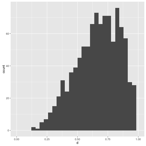
The central tendency of the posterior floats about 0.75, which is what we’d
expect, given our observations. This has been inferred from only four
points; let’s try adding a few more. But before we do that, note that the
present way the rejection sampling algorithm works is:
- Propose a parameter value according to the supplied proposal distribution.
- Generate a sample from the model, of equal size to the supplied observations.
- Compare the collected sample to the supplied observations. If they’re equal,
then return the proposed parameter value. Otherwise start over.
Rejection sampling isn’t exactly efficient in nontrivial settings anyway, but
it’s supremely inefficient for our present case. The random variables we’re
interested in are exchangeable, so what we’re concerned about is the
total number of True or False values observed - not any specific order they
appear in.
We can add an ‘assistance’ function to the rejection sampler to help us out in
this case:
invertWithAssistance
  :: (Monad m, Eq c) => ([a] -> c) -> m b -> (b -> m a) -> [a] -> m b
invertWithAssistance assister proposal model observed = loop where
  loop = do
    parameters <- proposal
    generated  <- replicateM (length observed) (model parameters)
    if   assister generated == assister observed
    then return parameters
    else loop
The assister summarizes both our observations and collected sample to ensure
they’re efficiently comparable. In our situation, we can use a simple counting
function to tally up the number of True values we observe:
count :: [Bool] -> Int
count = length . filter id
Now let’s create another posterior by conditioning on a few more observations:
posterior0 :: Model Double
posterior0 = invertWithAssitance count uniform bernoulli obs where
  obs =
    [True, True, True, False, True, True, False, True, True, True, True, False]
and collect another thousand samples from it. This would likely take an
annoying amount of time without the use of our count function for assistance
above:
> replicateM 1000 (simulate posterior0)
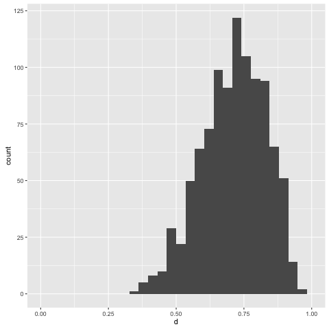
Note that with more information to condition on, we get a more informative
posterior.
Conclusion
This is a really basic formulation - too basic to be useful in any meaningful
way - but it illustrates some of the most important concepts in probabilistic
programming. Representation, simulation, and inference.
I think it’s also particularly nice to do this in Haskell, rather than something
like Python (which Dan used in his talk) - it provides us with a lot of
extensible structure in a familiar framework for language hacking. It sort of
demands you’re a fan of all these higher-kinded types and structured recursions
and all that, but if you’re reading this blog then you’re probably in that camp
anyway.
I’ll probably write a few more little articles like this over time. There are
a ton of improvements that we can make to this basic setup - encoding
independence, sampling via MCMC, etc. - and it might be fun to
grow everything out piece by piece.
I’ve dropped the code from this post into this gist.
01 Oct 2016
Randomness is a constant nuisance point for Haskell beginners who may be coming
from a language like Python or R. While in Python you can just get away with
something like:
In [2]: numpy.random.rand(3)
Out[2]: array([ 0.61426175,  0.05309224,  0.38861597])
or in R:
> runif(3)
[1] 0.49473012 0.68436352 0.04135914
In Haskell, the situation is more complicated. It’s not too much worse when
you get the hang of things, but it’s certainly one of those things that throws
beginners for a loop - and for good reason.
In this article I want to provide a simple guide, with examples, for getting
started and becoming comfortable with randomness in Haskell. Hopefully it
helps!
I’m writing this from a hotel during my girlfriend’s birthday, so it’s being
slapped together very rapidly with a kind of get-it-done attitude. If anything
is unclear or you have any questions, feel free to shoot me a ping and I’ll try
to improve it when I get a chance.
Randomness on Computers in General
Check out the R code I posted previously. If you just open R and type
runif(3) on your machine, then odds are you’ll get a different triple of
numbers than what I got above.
These numbers are being generated based on R’s global random number generator
(RNG), which, absent any fiddling by the user, is initialized as needed based
on the system time and ID of the R process. So: if you open up the R
interpreter and call runif(3), then behind the scenes R will initialize the
RNG based on the time and process ID, and then use a particular algorithm to
generate random numbers based on that initialized value (called the ‘seed’).
These numbers aren’t truly random - they’re pseudo-random, which means
they’re generated by a deterministic algorithm such that the resulting values
appear random over time. The default algorithm used by R, for example, is
the famous Mersenne Twister, which you can verify as follows:
> RNGkind()
[1] "Mersenne-Twister" "Inversion"
You can also set the seed yourself in R, using the set.seed function. Then
if you type something like runif(3), R will use this initialized RNG rather
than coming up with its own seed based on the time and process ID. Setting
the seed allows you to reproduce operations involving pseudo-random numbers;
just re-set the seed and perform the same operations again:
> set.seed(42)
> runif(3)
[1] 0.9148060 0.9370754 0.2861395
> set.seed(42)
> runif(3)
[1] 0.9148060 0.9370754 0.2861395
(It’s good practice to always initialize the RNG using some known seed before
running an experiment, simulation, and so on.)
So the big thing to notice here, in any case, is that R uses a global RNG.
It maintains the state of this RNG implicitly and behind the scenes. When you
type runif(3), R consults this implicit RNG, gives you your pseudo-random
numbers based on its value, and updates the global RNG without you needing to
worry about any of this plumbing yourself. The same is generally true for
randomness in most programming languages - Python, C, Ruby, and so on.
Explicit RNG Management
But let’s come back to Haskell. Haskell, unlike R or Python, is
purely-functional. State, or effects in general, are never implicit in the
same way that R updates its global RNG. We need to either explicitly pass
around a RNG ourselves, or at least allow some explicit monad to do it for us.
Passing around a RNG manually is annoying, so in practice this means everyone
uses a monad to handle RNG state. This means that one needs to be
comfortable working with monadic code in order to practically use random
numbers in Haskell, which presents a big hurdle for beginners who may have
been able to ignore monads thus far on their Haskell journey.
Let’s see what I mean by all of this by going through a few examples. Make
sure you have stack installed, and then grab a few libraries that we’ll
make use of in the remainder of this post:
$ stack install random mwc-random primitive
The Really Annoying Method - Manual RNG Management
Let me demonstrate the simplest conceptual method for dealing with random
numbers: manually grabbing and passing around a RNG without involving any
monads whatsoever.
First, open up GHCi:
And let’s also get some quick preliminaries out of the way:
Prelude> :set prompt "> "
> import System.Random
> import Control.Monad
> let runif_pure = randomR (0 :: Double, 1)
> let runif n = replicateM n (randomRIO (0 :: Double, 1))
> let set_seed = setStdGen . mkStdGen
We’ll first use the basic System.Random module for illustration. To
initialize a RNG, we can make one by providing the mkStdGen function
with an integer seed:
> let rng = mkStdGen 42
> rng
43 1
We can use this thing to generate random numbers. A simple function to do that
is randomR, which will generate pseudo-random values for some ordered
type in a given range. We’ll use the runif_pure alias for it that we defined
previously, just to make things look similar to the previous R example and also
emphasize that this one is a pure function:
> runif_pure rng
(1.0663729393723398e-2,2060101257 2103410263)
You can see that we got back a pair of values, the first element of which is
our random number 1.0663729393723398e-2. Cool. Let’s try to generate
another:
> runif_pure rng
(1.0663729393723398e-2,2060101257 2103410263)
Hmm. We generated the same number again. This is because the value of rng
hasn’t changed - it’s still the same value we made via mkStdGen 42. Since
we’re using the same random number generator to generate a pseudo-random value,
we get the same pseudo-random value.
If we want to make new random numbers, then we need to use a different
generator. And the second element of the pair returned from our call to
runif_pure is exactly that - an updated RNG that we can use to generate
additional random numbers.
Let’s try that all again, using the generator we get back from the first
function call as an input to the second:
> let (x, rng1) = runif_pure rng
> x
1.0663729393723398e-2
> let (y, rng2) = runif_pure rng1
> y
0.9827538369038856
Success!
I mean.. sort of. It works and all, and it does constitute a general-purpose
solution. But manually binding updated RNG states to names and swapping those
in for new values is still pretty annoying.
You could also generate an infinite list of random numbers using the
randomRs function and just take from it as needed, but you still
probably need to manage that list to make sure you don’t re-use any numbers.
You kind of trade off managing the RNG for managing an infinite list of random
numbers, which isn’t much better.
The Less-Annoying Method - Get A Monad To Do It
The good news is that we can offload the job of managing the RNG state to a
monad. I won’t actually explain how that works in detail here - I think most
people facing this problem are initially more concerned with getting something
working, rather than deeply grokking monads off the bat - so I’ll just claim
that we can get a monad to handle the RNG state for us, and that will hopefully
(mostly) suffice for now.

Still rolling with the System.Random module for the time being, we’ll use the
runif alias for the randomRIO function that we defined previously to
generate some new random numbers:
> runif 3
[0.9873934690803106,0.3794382930121829,0.2285653405908732]
> runif 3
[0.7651878964537555,0.2623159001635825,0.7683468476766804]
Simpler! Notice we haven’t had to do anything with a generator manually - we
just ask for random numbers and then get them, just like in R. And if we want
to set the value of the RNG being used here, we can use the setStdGen
function with an RNG that we’ve already created. Here let’s just use the
set_seed alias we defined earlier, to mimic R’s set.seed function:
> set_seed 42
> runif 3
[1.0663729393723398e-2,0.9827538369038856,0.7042944187434987]
> set_seed 42
> runif 3
[1.0663729393723398e-2,0.9827538369038856,0.7042944187434987]
So things are similar to how they work in R here - we have a global RNG of
sorts, and we can set its state as desired using the set_seed function. But
since this is Haskell, the effects of creating and updating the generator state
must still be explicit. And they are explicit - it’s just that they’re
explicit in the type of runif:
> :t runif
runif :: Int -> IO [Double]
Note that runif returns a value that’s wrapped up in IO. This is how we
indicate explicitly - at the type level - that something is being done with the
generator in the background. IO is a monad, and it happens to be the thing
that’s dealing with the generator for us here.
What this means for you, the practitioner, is that you can’t just mix values of
some type a with values of type IO a willy-nilly. You may be writing a
function f with type [Double] -> Double, where the input list of doubles is
intended to be randomly-generated. But if you just go ahead and generate a
list xs of random numbers, they’ll have type IO [Double], and you’ll stare
in confusion at some type error from GHC when you try to apply f to xs.
Here’s what I mean. Take the example of just generating some random numbers
and then summing them up. First, in R:
> xs = runif(3)
> sum(xs)
[1] 1.20353
And now in Haskell, using the same mechanism we tried earlier:
> let xs = runif 3
> :t xs
xs :: IO [Double]
> sum xs
<interactive>:16:1:
    No instance for (Num [Double]) arising from a use of ‘sum’
    In the expression: sum xs
    In an equation for ‘it’: it = sum xs
This means that to deal with the numbers we generate, we have to treat them a
little differently than we would in R, or compared to the situation where we
were managing the RNG explicitly in Haskell. Concretely: if we use a monad to
manage the RNG for us, then the numbers we generate will be ‘tagged’ by the
monad. So we need to do something or other to make those tagged numbers work
with ‘untagged’ numbers, or functions designed to work with ‘untagged’ numbers.
This is where things get confusing for beginners. Here’s how we could add up
some random numbers in GHCi:
> xs <- runif 3
> sum xs
1.512024272587933
We’ve used the <- symbol to bind the result of runif 3 to the name xs,
rather than let xs = .... But this is sort of particular to running code in
GHCi; if you try to do this in a generic Haskell function, you’ll possibly wind
up with some more weird type errors. To do this in regular ol’ Haskell code,
you need to both use <--style binding and also acknowledge the ‘tagged’
nature of randomly-generated values.
The crux is that, when you’re using a monad to generate random numbers in
Haskell, you need to separate generating them from using them. Rather than
try to explain what I mean here precisely, let’s rely on example, and implement
a simple Metropolis sampler for illustration.
A Metropolis Sampler
The Metropolis algorithm will help you approximate expectations over
certain probability spaces. Here’s how it works. Picture yourself strolling
around some bumpy landscape; you want to walk around it in such a fashion that
you visit regions of it with probability proportional to their altitude. To do
that, you can repeatedly:
- Pick a random point near your current location.
- Compare your present altitude to the altitude of that point you picked.
Calculate a probability based on their ratio.
- Flip a coin where the chance of observing a head is equal to that
probability. If you get a head, move to the location you picked.
Otherwise, stay put.
Let’s implement it in Haskell, using a monadic random number generator to do
so. This time we’re going to use mwc-random - a more industrial-strength
randomness library that you can confidently use in production code.
mwc-random uses Marsaglia’s multiply-with-carry algorithm to generate
pseudo-random numbers. It requires you to explicitly create and pass a RNG to
functions that need to generate random numbers, but it uses a monad to update
the RNG state itself. This winds up being pretty nice; let’s dive in to see.
Create a module called Metropolis.hs and get some imports out of the way:
module Metropolis where

import Control.Monad
import Control.Monad.Primitive
import System.Random.MWC as MWC
import System.Random.MWC.Distributions as MWC
Step One
The first thing we want to do is implement is point (1) from above:
Pick a random point near your current location.
We’ll just use a standard normal distribution of the appropriate dimension to
do this - we just want to take a location, perturb it, and return the perturbed
location.
propose :: [Double] -> Gen RealWorld -> IO [Double]
propose location rng = traverse (perturb rng) location where
  perturb gen x = MWC.normal x 1 gen
So at finer detail: we’re walking over the coordinates of the current location
and generating a normally-distributed value centered at each coordinate. The
MWC.normal function will do this for a given mean and standard
deviation, and we can use the traverse function to walk over each coordinate.
Note that we pass a mwc-random RNG - the value with type Gen RealWorld - to
the propose function. We need to supply this generator anywhere we want to
generate random numbers, but we don’t need to manually worry about tracking and
updating its state. The IO monad will do that for us. The resulting
randomly-generated values will be tagged with IO, so we’ll need to deal with
that appropriately.
Step Two
Now let’s implement point (2):
Compare your present altitude to the altitude of that point you picked.
Calculate a probability based on their ratio.
So, we need a function that will compare the altitude of our current point to
the altitude of a proposed point and compute a probability from that. The
following will do: it takes a function that will compute a (log-scale) altitude
for us, as well as the current and proposed locations, and returns a
probability.
moveProbability :: ([Double] -> Double) -> [Double] -> [Double] -> Double
moveProbability altitude current proposed =
    whenNaN 0 (exp (min 0 (altitude proposed - altitude current)))
  where
    whenNaN val x
      | isNaN x   = val
      | otherwise = x
Step Three
Finally, the third step of the algorithm:
Flip a coin where the chance of observing a head is equal to that
probability. If you get a head, move to the location you picked. Otherwise
stay put.
So let’s get to it:
decide :: [Double] -> [Double] -> Double -> Gen RealWorld -> IO [Double]
decide current proposed prob rng = do
  accept <- MWC.bernoulli prob rng
  return $
    if   accept
    then proposed
    else current
Here we need to flip a coin, so we require a source of randomness again. The
decide function thus takes another generator of type Gen RealWorld that we
then supply to the MWC.bernoulli function, and the result - the final
location - is once again wrapped in IO.
This function clearly demonstrates the typical way that you’ll deal with random
numbers in Haskell code. decide is a monadic function, so it proceeds using
do-notation. When you need to generate a random value - here we generate a
random True or False value according to a Bernoulli distribution - you bind
the result to a name using the <- symbol. Then afterwards, in the scope of
the function, you can use the bound value as if it were pure. But the entire
function must still return a ‘wrapped-up’ value that makes the effect of
passing the generator explicit at the type level; right here, that means that
the value will be wrapped up in IO.
Putting Everything Together
The final Metropolis transition is a combination of steps one through three.
We can put them together like so:
metropolis :: ([Double] -> Double) -> [Double] -> Gen RealWorld -> IO [Double]
metropolis altitude current rng = do
  proposed <- propose current rng
  let prob = moveProbability altitude current proposed
  decide current proposed prob rng
Again, metropolis is monadic, so we start off with a do to make monadic
programming easy on us. Whenever we need a random value, we bind the result of
a random number-returning function using the <- notation.
The propose function returns a random location, so we bind its result to the
name proposed using the <- symbol. The moveProbability function, on the
other hand, is pure - so we bind that using a let prob = ... expression. The
decide function returns a random value, so we can just plop it right on the
end here. The entire result of the metropolis function is random, so it is
wrapped up in IO.
The result of metropolis is just a single transition of the Metropolis
algorithm, which involves doing this kind of thing over and over. If we do
that, we observe a bunch of points that trace out a particular realization of a
Markov chain, which we can generate as follows:
chain
  :: Int -> ([Double] -> Double) -> [Double] -> Gen RealWorld -> IO [[Double]]
chain epochs altitude origin rng = loop epochs [origin] where
  loop n history@(current:_)
    | n <= 0    = return history
    | otherwise = do
        next <- metropolis altitude current rng
        loop (n - 1) (next:history)
An Example
Now that we have our chain function, we can use it to trace out a collection
of points visited on a realization of a Markov chain. Remember that we’re
supposed to be wandering over some particular abstract landscape; here, let’s
stroll over the one defined by the following function:
landscape :: [Double] -> Double
landscape [x0, x1] =
  -0.5 * (x0 ^ 2 * x1 ^ 2 + x0 ^ 2 + x1 ^ 2 - 8 * x0 - 8 * x1)
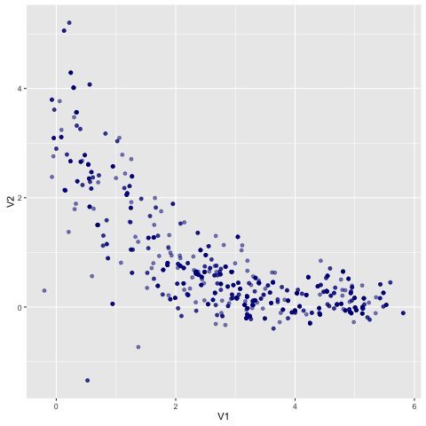
What we’ll now do is pick an origin to start from, wander over the landscape
for some number of steps, and then print the resulting realization of the
Markov chain to stdout. We’ll do all that through the following main
function:
main :: IO ()
main = do
  rng <- MWC.createSystemRandom
  let origin = [-0.2, 0.3]
  trace <- chain 1000 landscape origin rng
  mapM_ print trace
Running that will dump a trace to stdout. If you clean it up and plot it,
you’ll see that the visited points have traced out a rough approximation of the
landscape:
Fini
Hopefully this gives a broad idea of how to go about using random numbers in
Haskell. I’ve talked about:
- Why randomness in Haskell isn’t as simple as randomness in (say) Python or R.
- How to handle randomness in Haskell, either by manual generator management or
by offloading that job to a monad.
- How to get thing done when a monad manages the generator for you - separating
random number generation from random number processing.
- Doing all the above with an industrial-strength RNG, using a simple
Metropolis algorithm as an example.
Hopefully the example gives you an idea of how to work with random numbers in
practice.
I’ll be the first to admit that randomness in Haskell requires more work than
randomness in a language like R, which to this day remains my go-to interactive
data analysis language of choice. Using randomness effectively in Haskell
requires a decent understanding of how to work with monadic code, even if one
doesn’t quite understand monads entirely yet.
What I can say is that when one has developed some intuition for monads -
acquiring a ‘feel’ for how to work with monadic functions and values - the
difficulty and awkwardness drop off a bit, and working with randomness feels no
different than working with any other effect.
Happy generating! I’ve dumped the code for the Metropolis example into a
gist.
For a more production-quality Metropolis sampler, you can check out my
mighty-metropolis library, which is a member of the declarative
suite of MCMC algos.
18 Jul 2016
.. this one is pretty dry, I’ll admit. David Williams said it
best:
.. Measure theory, that most arid of subjects when done for its own sake,
becomes amazingly more alive when used in probability, not only because it is
then applied, but also because it is immensely enriched.
Unfortunately for you, dear reader, we won’t be talking about probability.
Moving on. What does it mean for something to be measurable in the
mathematical sense? Take some arbitrary collection \(X\) and slap an
appropriate algebraic structure \(\mathcal{X}\) on it - usually an
algebra or \(\sigma\)-algebra, etc. Then we can
refer to a few different objects as ‘measurable’, going roughly as follows.
The elements of the structure \(\mathcal{X}\) are called measurable sets.
They’re called this because they can literally be assigned a notion of measure,
whcih is a kind of generalized volume. If we’re just talking about some subset
of \(X\) out of the context of its structure then we can be pedantic and call
it measurable with respect to \(\mathcal{X}\), say. You could also call a
set \(\mathcal{X}\)-measurable, to be similarly precise.
The product of the original collection and its associated structure \((X,
\mathcal{X})\) is called a measurable space. It’s called that because it can
be completed with a measuring function \(\mu\) - itself called a measure - that
assigns notions of measure to measurable sets.
Now take some other measurable space \((Y, \mathcal{Y})\) and consider a
function \(f\) from \(X\) to \(Y\). This is a measurable function if it
satisfies the following technical requirement: that for any
\(\mathcal{Y}\)-measurable set, its preimage under \(f\) is an element of
\(\mathcal{X}\) (so: the preimage under \(f\) is \(\mathcal{X}\)-measurable).
The concept of measurability for functions probably feels the least intuitive
of the three - like one of those dry taxonomical classifications that we just
have to keep on the books. The ‘make sure your function is measurable and
everything will be ok’ heuristic will get you pretty far. But there is some
good intuition available, if you want to look for it.
Here’s an example: define a set \(X\) that consists of the elements \(A\),
\(B\), and \(C\). To talk about measurable functions, we first need to define
our measurable sets. The de-facto default structure used for this is a
\(\sigma\)-algebra, and we can always generate one from some
underlying class of sets. Let’s do that from the following plain old
partition that splits the original collection into a couple of disjoint
‘slices’:
\[H = \{\{A, B\}, \{C\}\}\]
The \(\sigma\)-algebra \(\mathcal{X}\) generated from this partition will just
be the partition itself, completed with the whole set \(X\) and the empty set.
To be clear, it’s the following:
\[\mathcal{X} = \left\{\{A, B, C\}, \{A, B\}, \{C\}, \emptyset\right\}\]
The resulting measurable space is \((X, \mathcal{X})\). So we could assign a
notion of generalized volume to any element of \(\mathcal{X}\), though I won’t
actually worry about doing that here.
Now. Let’s think about some functions from \(X\) to the real numbers, which
we’ll assume to be endowed with a suitable \(\sigma\)-algebra of their own (one
typically assumes the standard topology on \(\mathbb{R}\) and the
associated Borel \(\sigma\)-algebra).
How about this - a simple indicator function on the slice containing \(C\):
\[f(x) =
\begin{cases}
0, \, x \in \{A, B\} \\
1, \, x \in \{C\}
\end{cases}\]
Is it measurable? That’s easy to check. The preimage of \(\{0\}\) is \(\{A,
B\}\), the preimage of \(\{1\}\) is \(\{C\}\), and the preimage of \(\{0, 1\}\)
is \(X\) itself. Those are all in \(\mathcal{X}\), and the preimage of the
empty set is the empty set, so we’re good.
Ok. What about this one:
\[g(x) =
\begin{cases}
0, \, x \in \{A\} \\
1, \, x \in \{B\} \\
2, \, x \in \{C\}
\end{cases}\]
Check the preimage of \(\{1, 2\}\) and you’ll find it’s \(\{B, C\}\). But
that’s not a member of \(\mathcal{X}\), so \(g\) is not measurable!
What happened here? Failing to satisfying technical requirements aside: what,
intuitively, made \(f\) measurable where \(g\) wasn’t?
The answer is a problem of resolution. Look again at \(\mathcal{X}\):
\[\left\{\{A, B, C\}, \{A, B\}, \{C\}, \emptyset\right\}\]
The structure \(\mathcal{X}\) that we’ve endowed our collection \(X\) with is
too coarse to permit distinguishing between elements of the slice \(\{A,
B\}\). There is no measurable set \(A\), nor a measurable set \(B\) - just
a measurable set \(\{A, B\}\). And as a result, if we define a function that
says something about either \(A\) or \(B\) without saying the same thing about
the other, that function won’t be measurable. The function \(f\) assigned
the same value to both \(A\) and \(B\), so we didn’t have any problem there.
If we want to be able to distinguish between \(A\) and \(B\), we’ll need to
equip \(X\) with some structure that has a finer resolution. You can check
that if you make a measurable space out of \(X\) and its power set (the set of
all subsets of \(X\)) then \(g\) will be measurable there, for example.
So if we’re using partitions to define our measurable sets, we get a neat
little property: for any measurable function, elements in the same slice of the
partition must have the same value when passed through the function. So if
you have a function \(h : X \to H\) that takes an element to its respective
slice in a partition, you know that \(h(x_{0}) = h(x_{1})\) for any \(x_{0}\),
\(x_{1}\) in \(X\) implies that \(f(x_{0}) = f(x_{1})\) for any measurable
function \(f\).
Addendum
Whipping together a measurable space using a \(\sigma\)-algebra generated by a
partition of sets occurs naturally when we talk about correlated
equilibrium, a solution concept in non-cooperative game theory. It’s
common to say a function - in that context a correlated strategy - must be
measurable ‘with respect to the partition’, which sort of elides the fact that
we still need to generate a \(\sigma\)-algebra from it anyway.
Some oldschool authors (Halmos, at least) developed their measure theory using
\(\sigma\)-rings, but this doesn’t seem very popular nowadays.
Since a ring doesn’t require including the entire set \(X\), you need to go
through an awkward extra hoop when defining measurability on functions. But
regardless, it’s interesting to think about what happens when one uses
different structures to define measurable sets!