Markov Chains à la Carte

I’ve released a number of libraries for doing Markov Chain Monte Carlo (MCMC) in Haskell.

You can get at them via a ‘frontend’ library, declarative, but each can also be used fruitfully on its own. À la carte, if you will.

Some background: MCMC is a family of stateful algorithms for sampling from a large class of probability distributions. Typically one is interested in doing this to approximate difficult integrals; instead of choosing some suitable grid of points in parameter space over which to approximate an integral, just offload the problem to probability theory and use a Markov chain to find them for you.

For an excellent introduction to MCMC you won’t find better than Iain Murray’s lectures from MLSS ’09 in Cambridge, so check those out if you’re interested in more details.

I’ve put together a handful of popular MCMC algorithms as well as an easy way to glue them together in a couple of useful ways. At present these implementations are useful in cases where you can write your target function in closed form, and that’s pretty much all that’s required (aside from the standard algorithm-specific tuning parameters).

The API should be pretty easy to work with — write your target as a function of its parameters, specify a start location, and away you go. It’s also cool if your target accepts its parameters via most common traversable functors — lists, vectors, sequences, maps, etc.

That’s sort of the goal of this first release: if you can give me a target function, I’ll do my best to give you samples from it. Less is more and all that.

What‘s In The Box

There are a number of libraries involved. I have a few more in the queue and there are a number of additional features I plan to support for these ones in particular, but without further ado:

• mwc-probability, a sampling-function based probability monad implemented as a thin wrapper over the excellent mwc-random library.
• mcmc-types, housing a number of types used by the the whole family.
• mighty-metropolis, an implementation of the famous Metropolis algorithm.
• speedy-slice, a slice sampling implementation suitable for both continuous & discrete parameter spaces.
• hasty-hamiltonian, an implementation of the gradient-based Hamiltonian Monte Carlo algorithm.
• declarative, the one ring to rule them all.

Pull down declarative if you just want to have access to all of them. If you’re a Haskell neophyte you can find installation instructions at the Github repo.

Motivation

MCMC is fundamentally about observing Markov chains over probability spaces. In this context a chain is a stochastic process that wanders around a state space, eventually visiting regions of the space in proportion to their probability.

Markov chains are constructed by transition operators that obey the Markov property: that the probability of transitioning to the next location — conditional on the history of the chain — depends only on the current location. For MCMC we’re also interested in operators that satisfy the reversibility property — that the probability a transition from state A to state B occurs is the same as that a transition from state B to state A occurs. A chain is characterized by a transition operator T that drives it from state to state, and for MCMC we want the stationary or limiting distribution of the chain to be the distribution we’re sampling from.

One of the major cottage industries in Bayesian research is inventing new transition operators to drive the Markov chains used in MCMC. This has been fruitful, but it could likely be aided by a practical way to make existing transition operators work together.

This is easy to do in theory: there are a couple of ways to combine transition operators such that the resulting composite operator preserves all the properties we’re interested in for MCMC — the stationary distribution, reversibility, and Markov property. See Geyer, 2005 for details here, but the crux is that we can establish the following simple grammar for transition operators:

transition ::= primitive <transition>
             | concat transition transition
             | sample transition transition

A transition is either some primitive operator, a deterministic concatenation of operators (via ‘concat’), or a probabilistic concatenation of operators (via ‘sample’). A deterministic concatenation works by just transitioning through two operators one after the other; a probabilistic concatenation works by randomly choosing one transition operator or the other to use on any given transition. These kinds of concatenation preserve all the properties we’re interested in.

We can trivially generalize this further by adding a term that concatenates n transition operators together deterministically, or another for probabilistically concatenating a bunch of operators according to some desired probability distribution.

The idea here is that there are tradeoffs involved in different transition operators. Some may be more computationally expensive than others (perhaps requiring a gradient evaluation, or evaluation of some inner loop) but have better ability to make ‘good’ transitions in certain situations. Other operators are cheap, but can be inefficient (taking a long time to visit certain regions of the space).

By employing deterministic or probabilistic concatenation, one can concoct a Markov chain that uses a varied range of tuning parameters, for example. Or only occasionally employs a computationally expensive transition, otherwise preferring some cheaper, reliable operator.

Usage

The declarative library implements this simple language for transition operators, and the mighty-metropolis, speedy-slice, and hasty-hamiltonian libraries provide some primitive transitions that you can combine as needed.

The Metropolis and slice sampling transitions are cheap and require little information, whereas Hamiltonian Monte Carlo exploits information about the target’s gradient and also involves evaluation of an inner loop (the length of which is determined by a tuning parameter). Feel free to use one that suits your problem, or combine them together using the combinators supplied in declarative to build a custom solution.

As an example, the Rosenbrock density is a great test dummy as it’s simple, low-dimensional, and can be easily visualized, but it still exhibits a pathological anisotropic structure that makes it somewhat tricky to sample from.

Getting started via declarative is pretty simple:

import Numeric.MCMC

You’ll want to supply a target to sample over, and if you want to use an algorithm like Hamiltonian Monte Carlo you’ll also need to provide a gradient. If you can’t be bothered to calculate gradients by hand, you can always turn to your friend automatic differentiation:

import Numeric.AD

The Rosenbrock log-density and its gradient can then be written as follows:

target :: Num a => [a] -> a
target [x0, x1] = negate (100 * (x1 — x0 ^ 2) ^ 2 + (1 — x0) ^ 2)

gTarget :: Num a => [a] -> [a]
gTarget = grad target

All you need to do here is provide a function proportional to a log-probability density. The logarithmic scale is important; various internals expect to be passed (something proportional to) a log-probability density.

To package these guys up together we can wrap them in a Target. Note that we don’t always care about including a gradient, so that part is optional:

rosenbrock :: Target [Double]
rosenbrock = Target target (Just gTarget)

The Target type is parameterized over the shape of the parameter space. You could similarly have a Target (Seq Double), Target (Map String Double), and so on. Your target may be implemented using a boxed vector for efficiency, for example. Or using a Map or HashMap with string/text keys such that parameter names are preserved. They should work just fine.

Given a target, we can sample from it a bunch of times using a simple Metropolis transition via the mcmc function. Aside from the target and a PRNG, provide it with the desired number of transitions, a starting point, and the transition operator to use:

> -- haskell
> prng <- create
> mcmc 10000 [0, 0] (metropolis 1) rosenbrock prng

In return you’ll get the desired trace of the chain dumped to stdout:

8.136972300105949e-2,0.273896953404261
0.4657348148676972,0.17462596647788464
-0.48609414127836326,9.465052854751566e-2
-0.49781488399832785,0.42092910345708523
-0.3019713424699155,0.39135350029173566
0.12058426470979189,0.12485407390388925
..

The intent is for the chain to be processed elsewhere — if you’re me, that will usually be in R. Libraries like coda have a ton of functionality useful for working with Markov chain traces, and ggplot2 as a library for static statistical graphics can’t really be beat:

> # r
> d = read.csv(‘rosenbrock-trace.dat’, header = F)
> names(d) = c(‘x’, ‘y’)
> require(ggplot2)
> ggplot(d, aes(x, y)) + geom_point(colour = ‘darkblue’, alpha = 0.2)

You get the following trace over the Rosenbrock density, taken for 10k iterations. This is using a Metropolis transition with variance 1:

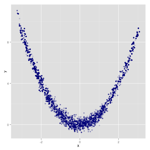
If you do want to work with chains in memory in Haskell you can do that by writing your own handling code around the supplied transition operators. I’ll probably make this a little easier in later versions.

The implementations are reasonably quick and don’t leak memory — the traces are streamed to stdout as the chains are traversed. Compiling the above with ‘-O2’ and running it for 100k iterations yields the following performance characteristics on my mid-2011 model MacBook Air:

$ ./test/Rosenbrock +RTS -s > /dev/null

3,837,201,632 bytes allocated in the heap
    8,453,696 bytes copied during GC
       89,600 bytes maximum residency (2 sample(s))
       23,288 bytes maximum slop
         1 MB total memory in use (0 MB lost due to fragmentation)

 INIT time 0.000s ( 0.000s elapsed)
  MUT time 3.539s ( 3.598s elapsed)
   GC time 0.049s ( 0.058s elapsed)
 EXIT time 0.000s ( 0.000s elapsed)
Total time 3.591s ( 3.656s elapsed)

%GC time 1.4% (1.6% elapsed)

Alloc rate 1,084,200,280 bytes per MUT second

Productivity 98.6% of total user, 96.8% of total elapsed

The beauty is that rather than running a chain solely on something like the simple Metropolis operator used above, you can sort of ‘hedge your sampling risk’ and use a composite operator that proposes transitions using a multitude of ways. Consider this guy, for example:

transition =
  concatT
    (sampleT (metropolis 0.5) (metropolis 1.0))
    (sampleT (slice 2.0) (slice 3.0))

Here concatT and sampleT correspond to the concat and sample terms in the BNF description in the previous section. This operator performs two transitions back-to-back; the first is randomly a Metropolis transition with standard deviation 0.5 or 1 respectively, and the second is a slice sampling transition using a step size of 2 or 3, randomly.

Running it for 5000 iterations (to keep the total computation approximately constant), we see a chain that has traversed the space a little better:

> mcmc 5000 [0, 0] transition rosenbrock prng

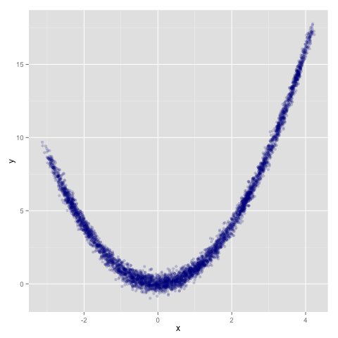
It’s worth noting that I didn’t put any work into coming up with this composite transition: this was just the first example I thought up, and a lot of the benefits here probably come primarily from including the eminently-reliable slice sampling transition. But from informal experimentation, it does seem that chains driven by composite transitions involving numerous operators and tuning parameter settings often seem to perform better on average than a given chain driven by a single (poorly-selected) transition.

I know exactly how meticulous proofs and benchmarks must be so I haven’t rigorously established any properties around this, but hey: it ‘seems to be the case’, and intuitively, including varied transition operators surely hedges your bets when compared to using a single one.

Try it out and see how your mileage varies, and be sure to let me know if you find some killer apps where composite transitions really seem to win.

Implementation Notes

If you’re just interested in using the libraries you can skip the following section, but I just want to point out how easy this is to implement.

The implementations are defined using a small set of types living in mcmc-types:

type Transition m a = StateT a (Prob m) ()

data Chain a b = Chain {
    chainTarget   :: Target a
  , chainScore    :: Double
  , chainPosition :: a
  , chainTunables :: Maybe b
  }

data Target a = Target {
    lTarget  :: a -> Double
  , glTarget :: Maybe (a -> a)
  }

Most important here is the Transition type, which is just a state transformer over a probability monad (itself defined in mwc-probability). The probability monad is the source of randomness used to define transition operators useful for MCMC, and values with type Transition are the transition operators in question.

The Chain type is the state of the Markov chain at any given iteration. All that’s really required here is the chainPosition field, which represents the location of the chain in parameter space. But adding some additional information here is convenient; chainScore caches the most recent score of the chain (which is typically used in internal calculations, and caching avoids recomputing things needlessly) and chainTunables is an optional record intended to be used for stateful tuning parameters (used by adaptive algorithms or in burn-in phases and the like). Additionally the target being sampled from itself — chainTarget — is included in the state.

Undisciplined use of chainTarget and chainTunables can have all sorts of nasty consequences — you can use them to change the stationary distribution you’re sampling from or invalidate the Markov property — but keeping them around is useful for implementing some desirable features. Tweaking chainTarget, for example, allows one to easily implement annealing, which can be very useful for sampling from annoying multi-modal densities.

Setting everything up like this makes it trivial to mix-and-match transition operators as required — the state and probability monad stack provides everything we need. Deterministic concatenation is implemented as follows, for example:

concatT = (>>)

and a generalized version of probabilistic concatenation just requires a coin flip:

bernoulliT p t0 t1 = do
  heads <- lift (MWC.bernoulli p)
  if heads then t0 else t1

A uniform probabilistic concatenation over two operators, implemented in sampleT, is then just bernoulliT 0.5.

The difficulty of implementing primitive operators just depends on the operator itself; the surrounding framework is extremely lightweight. Here’s the Metropolis transition, for example (with type signatures omitted to keep the noise down):

metropolis radial = do
  Chain {..} <- get
  proposal   <- lift (propose radial chainPosition)
  let proposalScore = lTarget chainTarget proposal
      acceptProb    = whenNaN 0
        (exp (min 0 (proposalScore - chainScore)))

  accept <- lift (MWC.bernoulli acceptProb)
  when accept
    (put (Chain chainTarget proposalScore proposal chainTunables))

propose radial = traverse perturb where
  perturb m = MWC.normal m radial

And the excellent pipes library is used to generate a Markov chain:

chain radial = loop where
  loop state prng = do
    next <- lift
      (MWC.sample (execStateT (metropolis radial) state) prng)
    yield next
    loop next prng

The mcmc functions are also implemented using pipes. Take the first n iterations of a chain and print them to stdout. That simple.

Future Work

In the near term I plan on updating some old MCMC implementations I have kicking around on Github (flat-mcmc, lazy-langevin, hnuts) and releasing them within this framework. Additionally I’ve got some code for building annealed operators that I want to release — it has been useful in some situations when sampling from things like the Himmelblau density, which has a few disparate clumps of probability that make it tricky to sample from with conventional algorithms.

This framework is also useful as an inference backend to languages for working with directed graphical models (think BUGS/Stan). The idea here is that you don’t need to specify your target function (typically a posterior density) explicitly: just describe your model and I’ll give you samples from the posterior distribution. A similar version has been put to use around the BayesHive project.

Longer term — I’ll have to see what’s up in terms of demand. There are performance improvements and straightforward extensions to things like parallel tempering, but I’m growing more interested in ‘online’ methods like particle MCMC and friends that are proving useful for inference in more general probabilistic programs (think those expressible by Church and its ilk).

Let me know if you get any use out of these things, or please file an issue if there’s some particular feature you’d like to see supported.

Thanks to Niffe Hermansson for review and helpful comments.