Comonadic Markov Chain Monte Carlo

Some time ago I came across a way to in-principle perform inference on certain probabilistic programs using comonadic structures and operations.

I decided to dig it up and try to use it to extend the simple probabilistic programming language I talked about a few days ago with a stateful, experimental inference backend. In this post we’ll

• Represent probabilistic programs as recursive types parameterized by a terminating instruction set.
• Represent execution traces of probabilistic programs via a simple transformation of our program representation.
• Implement the Metropolis-Hastings algorithm over this space of execution traces and thus do some inference.

Let’s get started!

Representing Programs That Terminate

I like thinking of embedded languages in terms of instruction sets. That is: I want to be able to construct my embedded language by first defining a collection of abstract instructions and then using some appropriate recursive structure to represent programs over that set.

In the case of probabilistic programs, our instructions are probability distributions. Last time we used the following simple instruction set to define our embedded language:

data ModelF r =
    BernoulliF Double (Bool -> r)
  | BetaF Double Double (Double -> r)
  deriving Functor

We then created an embedded language by just wrapping it up in the higher-kinded Free type to denote programs of type Model.

data Free f a =
    Pure a
  | Free (f (Free f a))

type Model = Free ModelF

Recall that Free represents programs that can terminate, either by some instruction in the underlying instruction set, or via the Pure constructor of the Free type itself. The language defined by Free ModelF is expressive enough to easily construct a ‘forward-sampling’ interpreter, as well as a simple rejection sampler for performing inference.

Notice that we don’t have a terminating instruction in ModelF itself - if we’re using it, then we need to rely on the Pure constructor of Free to terminate programs. Otherwise they’d just have to recurse forever. This can be a bit limiting if we want to transform a program of type Free ModelF to something else that doesn’t have a notion of termination baked-in (Fix, for example).

Let’s tweak the ModelF type to get the following:

data ModelF a r =
    BernoulliF Double (Bool -> r)
  | BetaF Double Double (Double -> r)
  | NormalF Double Double (Double -> r)
  | DiracF a
  deriving Functor

Aside from adding another foundational distribution - NormalF - we’ve also added a new constructor, DiracF, which carries a parameter with type a. We need to incorporate this carrier type in the overall type of ModelF as well, so ModelF itself also gets a new type parameter to carry around.

The DiracF instruction is a terminating instruction; it has no recursive point and just terminates with a value of type a when reached. It’s structurally equivalent to the Pure a branch of Free that we were relying on to terminate our programs previously - the only thing we’ve done is add it to our instruction set proper.

Why DiracF? A Dirac distribution places the entirety of its probability mass on a single point, and this is the exact probabilistic interpretation of the applicative pure or monadic return that one encounters with an appropriate probability type. Intuitively, if I sample a value \(x\) from a uniform distribution, then that is indistinguishable from sampling \(x\) from said uniform distribution and then sampling from a Dirac distribution with parameter \(x\).

Make sense? If not, it might be helpful to note that there is no difference between any of the following (to which uniform and dirac are analogous):

> action :: m a
> action >>= return :: m a
> action >>= return >>= return >>= return :: m a

Wrapping ModelF a up in Free, we get the following general type for our programs:

type Program a = Free (ModelF a)

And we can construct a bunch of embedded language terms in the standard way:

beta :: Double -> Double -> Program a Double
beta a b = liftF (BetaF a b id)

bernoulli :: Double -> Program a Bool
bernoulli p = liftF (BernoulliF p id)

normal :: Double -> Double -> Program a Double
normal m s = liftF (NormalF m s id)

dirac :: a -> Program a b
dirac x = liftF (DiracF x)

Program is a general type, capturing both terminating and nonterminating programs via its type parameters. What do I mean by this? Note that in Program a b, the a type parameter can only be concretely instantiated via use of the terminating dirac term. On the other hand, the b type parameter is unaffected by the dirac term; it can only be instantiated by the other nonterminating terms: beta, bernoulli, normal, or compound expressions of these.

We can thus distinguish between terminating and nonterminating programs at the type level, like so:

type Terminating a = Program a Void

type Model b = forall a. Program a b

Void is the uninhabited type, brought into scope via Data.Void or simply defined via data Void = Void Void. Any program that ends via a dirac instruction must be Terminating, and any program that doesn’t end with a dirac instruction can not be Terminating. We’ll just continue to call a nonterminating program a Model, as before.

Good. So if it’s not clear: from a user’s perspective, nothing has changed. We still write probabilistic programs using simple monadic language terms. Here’s a Gaussian mixture model where the mixing parameter follows a beta distribution, for example:

mixture :: Double -> Double -> Model Double
mixture a b = do
  prob   <- beta a b
  accept <- bernoulli prob
  if   accept
  then normal (negate 2) 0.5
  else normal 2 0.5

Meanwhile the syntax tree generated looks something like the following. It’s more or less a traditional probabilistic graphical model description of our program:

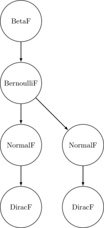
It’s important to note that in this embedded framework, the only pieces of the syntax tree that we can observe are those related directly to our primitive instructions. For our purposes this is excellent - we can focus on programs entirely at the level of their probabilistic components, and ignore the deterministic parts that would otherwise be distractions.

To collect samples from mixture, we can first interpret it into a sampling function, and then simulate from it. The toSampler function from last time doesn’t change much:

toSampler :: Program a a -> Prob IO a
toSampler = iterM $ \case
  BernoulliF p f -> Prob.bernoulli p >>= f
  BetaF a b f    -> Prob.beta a b >>= f
  NormalF m s f  -> Prob.normal m s >>= f
  DiracF x       -> return x

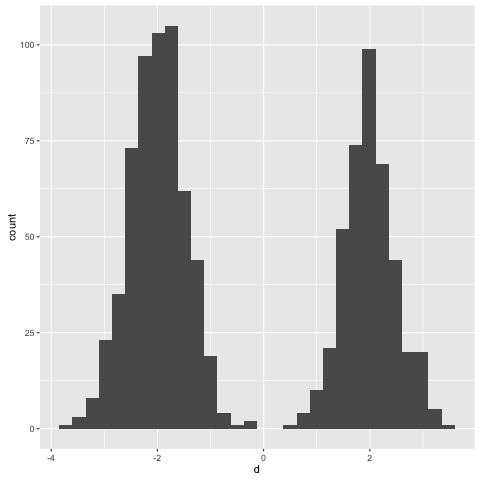
Sampling from mixture 2 3 a thousand times yields the following

> simulate (toSampler (mixture 2 3))

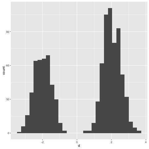
Note that the rightmost component gets more traffic due to the hyperparameter combination of 2 and 3 that we provided to mixture.

Also, a note - since we have general recursion in Haskell, so-called ‘terminating’ programs here can actually.. uh, fail to terminate. They must only terminate as far as we can express the sentiment at the embedded language level. Consider the following, for example:

foo :: Terminating a
foo = (loop 1) >>= dirac where
  loop a = do
    p <- beta a 1
    loop p

foo here doesn’t actually terminate. But at least this kind of weird case can be picked up in the types:

> :t simulate (toSampler foo)
simulate (toSampler foo) :: IO Void

If you try to sample from a distribution over Void or forall a. a then I can’t be held responsible for what you get up to. But there are other cases, sadly, where we’re also out of luck:

trollGeometric :: Double -> Model Int
trollGeometric p = loop where
  loop = do
    accept <- return False
    if   accept
    then return 1
    else fmap succ loop

A geometric distribution that actually used its argument \(p\), for \(0 < p \leq 1\), could be guaranteed to terminate with probability 1. This one doesn’t, so trollGeometric undefined >>= dirac won’t.

At the end of the day we’re stuck with what our host language offers us. So, take the termination guarantees for our embedded language with a grain of salt.

Stateful Inference

In the previous post we used a simple rejection sampler to sample from a conditional distribution. ‘Vanilla’ Monte Carlo algorithms like rejection and importance sampling are stateless. This makes them nice in some ways - they tend to be simple to implement and are embarrassingly parallel, for example. But the curse of dimensionality prevents them from scaling well to larger problems. I won’t go into detail on that here - for a deep dive on the topic, you probably won’t find anything better than this phenomenal couple of talks on MCMC that Iain Murray gave at a MLSS session in Cambridge in 2009. I think they’re unparalleled to this day.

The point is that in higher dimensions we tend to get a lot out of state. Essentially, if one finds an interesting region of high-dimensional parameter space, then it’s better to remember where that is, rather than forgetting it exists as soon as one stumbles onto it. The manifold hypothesis conjectures that interesting regions of space tend to be near other interesting regions of space, so exploring neighbourhoods of interesting places tends to pay off. Stateful Monte Carlo methods - namely, the family of Markov chain Monte Carlo algorithms - handle exactly this, by using a Markov chain to wander over parameter space. I’ve written on MCMC in the past - you can check out some of those articles if you’re interested.

In the stateless rejection sampler we just performed conditional inference via the following algorithm:

• Sample from a parameter model.
• Sample from a data model, using the sample from the parameter model as input.
• If the sample from the data model matches the provided observations, return the sample from the parameter model.

By repeating this many times we get a sample of arbitrary size from the appropriate conditional, inverse, or posterior distribution (whatever you want to call it).

In a stateful inference routine - here, the good old Metropolis-Hastings algorithm - we’re instead going to do the following repeatedly:

• Sample from a parameter model, recording the way the program executed in order to return the sample that it did.
• Compute the cost, in some sense, of generating the provided observations, using the sample from the parameter model as input.
• Propose a new sample from the parameter model by perturbing the way the program executed and recording the new sample the program outputs.
• Compute the cost of generating the provided observations using this new sample from the parameter model as input.
• Compare the costs of generating the provided observations under the respective samples from the parameter models.
• With probability depending on the ratio of the costs, flip a coin. If you see a head, then move to the new, proposed execution trace of the program. Otherwise, stay at the old execution trace.

This procedure generates a Markov chain over the space of possible execution traces of the program - essentially, plausible ways that the program could have executed in order to generate the supplied observations.

Implementations of Church use variations of this method to do inference, the most famous of which is a low-overhead transformational compilation procedure described in a great and influential 2011 paper by David Wingate et al.

Representing Running Programs

To perform inference on probabilistic programs according to the aforementioned Metropolis-Hastings algorithm, we need to represent executing programs somehow, in a form that enables us to examine and modify their internal state.

How can we do that? We’ll pluck another useful recursive structure from our repertoire and consider the humble Cofree:

data Cofree f a = a :< f (Cofree f a)

Recall that Cofree allows one to annotate programs with arbitrary information at each internal node. This is a great feature; if we can annotate each internal node with important information about its state - its current value, the current state of its generator, the ‘cost’ associated with it - then we can walk through the program and examine it as required. So, it can capture a ‘running’ program in exactly the way we need.

Let’s describe running programs as values having the following Execution type:

type Execution a = Cofree (ModelF a) Node

The Node type is what we’ll use to describe the internal state of each node on the program. I’ll define it like so:

data Node = Node {
    nodeCost    :: Double
  , nodeValue   :: Dynamic
  , nodeSeed    :: MWC.Seed
  , nodeHistory :: [Dynamic]
  } deriving Show

I’ll elaborate on this type below, but you can see that it captures a bunch of information about the state of each node.

One can mechanically transform any Free-encoded program into a Cofree-encoded program, so long as the original Free-encoded program can terminate of its own accord, i.e. on the level of its own instructions. Hence the need for our Terminating type and all that.

In our case, setting everything up just right takes a bit of code, mainly around handling pseudo-random number generators in a pure fashion. So I won’t talk about every little detail of it right here. The general idea is to write a function that takes instructions to the appropriate state captured by a Node value, like so:

initialize :: Typeable a => MWC.Seed -> ModelF a b -> Node
initialize seed = \case
  BernoulliF p _ -> runST $ do
    (nodeValue, nodeSeed) <- samplePurely (Prob.bernoulli p) seed
    let nodeCost    = logDensityBernoulli p (unsafeFromDyn nodeValue)
        nodeHistory = mempty
    return Node {..}

  BetaF a b _ -> runST $ do
    (nodeValue, nodeSeed) <- samplePurely (Prob.beta a b) seed
    let nodeCost    = logDensityBeta a b (unsafeFromDyn nodeValue)
        nodeHistory = mempty
    return Node {..}

  ...

You can see that for each node, I sample from it, calculate its cost, and then initialize its ‘history’ as an empty list.

Here it’s worth going into a brief aside.

There are two mildly annoying things we have to deal with in this situation. First, individual nodes in the program typically sample values at different types, and second, we can’t easily use effects when annotating. This means that we have to pack heterogeneously-typed things into a homogeneously-typed container, and also use pure random number generation facilities to sample them.

A quick-and-dirty answer for the first case is to just use dynamic typing when storing the values. It works and is easy, but of course is subject to the standard caveats. I use a function called unsafeFromDyn to convert dynamically-typed values back to a typed form, so you can gauge the safety of all this for yourself.

For the second case, I just use the ST monad, along with manual state snapshotting, to execute and iterate a random number generator. Pretty simple.

Also: in terms of efficiency, keeping a node’s history on-site at each execution falls into the ‘completely insane’ category, but let’s not worry much about efficiency right now. Prototypes gonna prototype and all that.

Anyway.

Given this initialize function, we can transform a terminating program into a running program by simple recursion. Again, we can only transform programs with type Terminating a because we need to rule out the case of ever visiting the Pure constructor of Free. We handle that by the absurd function provided by Data.Void:

execute :: Typeable a => Terminating a -> Execution a
execute = annotate defaultSeed where
  defaultSeed         = (42, 108512)
  annotate seeds term = case term of
    Pure r -> absurd r
    Free instruction ->
      let (nextSeeds, generator) = xorshift seeds
          seed  = MWC.toSeed (V.singleton generator)
          node  = initialize seed instruction
      in  node :< fmap (annotate nextSeeds) instruction

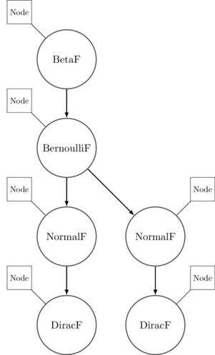
And there you have it - execute takes a terminating program as input and returns a running program - an execution trace - as output. The syntax tree we had previously gets turned into something like this:

Perturbing Running Programs

Given an execution trace, we’re able to step through it sequentially and investigate the program’s internal state. But to do inference we also need to modify it as well. What’s the answer here?

Just as Free has a monadic structure that allows us to write embedded programs using built-in monadic combinators and do-notation, Cofree has a comonadic structure that is amenable to use with the various comonadic combinators found in Control.Comonad. The most important for our purposes is the comonadic ‘extend’ operation that’s dual to monad’s ‘bind’:

extend :: Comonad w => (w a -> b) -> w a -> w b
extend f = fmap f . duplicate

To perturb a running program, we can thus write a function that perturbs any given annotated node, and then extend it over the entire execution trace.

The perturbNode function can be similar to the initialize function from earlier; it describes how to perturb every node based on the instruction found there:

perturbNode :: Execution a -> Node
perturbNode (node@Node {..} :< cons) = case cons of
  BernoulliF p _ -> runST $ do
    (nvalue, nseed) <- samplePurely (Prob.bernoulli p) nodeSeed
    let nscore   = logDensityBernoulli p (unsafeFromDyn nvalue)
    return $! Node nscore nvalue nseed nodeHistory

  BetaF a b _ -> runST $ do
    (nvalue, nseed) <- samplePurely (Prob.beta a b) nodeSeed
    let nscore   = logDensityBeta a b (unsafeFromDyn nvalue)
    return $! Node nscore nvalue nseed nodeHistory

  ...

Note that this is a very crude way to perturb nodes - we’re just sampling from whatever distribution we find at each one. A more refined procedure would sample from each node on a more local basis, sampling from its respective domain in a neighbourhood of its current location. For example, to perturb a BetaF node we might sample from a tiny Gaussian bubble around its current location, repeating the process if we happen to ‘fall off’ the support. I’ll leave matters like that for another post.

Perturbing an entire trace is then as easy as I claimed it to be:

perturb :: Execution a -> Execution a
perturb = extend perturbNode

For some comonadic intuition: when we ‘extend’ a function over an execution, the trace itself gets ‘duplicated’ in a comonadic context. Each node in the program becomes annotated with a view of the rest of the execution trace from that point forward. It can be difficult to visualize at first, but I reckon the following image is pretty faithful:

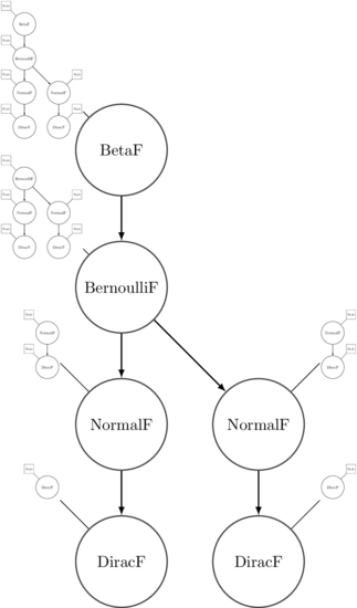
Each annotation then has perturbNode applied to it, which reduces the trace back to the standard annotated version we saw before.

Iterating the Markov Chain

So: to move around in parameter space, we’ll propose state changes by perturbing the current state, and then accept or reject proposals according to local economic conditions.

If you already have no idea what I’m talking about, then the phrase ‘local economic conditions’ probably didn’t help you much. But it’s a useful analogy to have in one’s head. Each state in parameter space has a cost associated with it - the cost of generating the observations that we’re conditioning on while doing inference. If certain parameter values yield a data model that is unlikely to generate the provided observations, then those observations will be expensive to generate when measured in terms of log-likelihood. Parameter values that yield data models more likely to generate the supplied observations will be comparatively cheaper.

If a proposed execution trace is significantly cheaper than the trace we’re currently at, then we usually want to move to it. We allow some randomness in our decision to keep everything nice and measure-preserving.

We can thus construct the conditional distribution over execution traces using the following invert function, using the same nomenclature as the rejection sampler we used previously. To focus on the main points, I’ll elide some of its body:

invert
  :: (Eq a, Typeable a, Typeable b)
  => Int -> [a] -> Model b -> (b -> a -> Double)
  -> Model (Execution b)
invert epochs obs prior ll = loop epochs (execute terminated) where
  terminated = prior >>= dirac
  loop n current
    | n == 0    = return current
    | otherwise = do
        let proposal = perturb current

            -- calculate costs and movement probability here

        accept <- bernoulli prob
        let next = if accept then proposal else stepGenerators current
        loop (pred n) (snapshot next)

There are a few things to comment on here.

First, notice how the return type of invert is Model (Execution b)? Using the semantics of our embedded language, it’s literally a standard model over execution traces. The above function returns a first-class value that is completely uninterpreted and abstract. Cool.

We’re also dealing with things a little differently from the rejection sampler that we built previously. Here, the data model is expressed by a cost function; that is, a function that takes a parameter value and observation as input, and returns the cost of generating the observation (conditional on the supplied parameter value) as output. This is the approach used in the excellent Practical Probabilistic Programming with Monads paper by Adam Scibior et al and also mentioned by Dan Roy in his recent talk at the Simons Institute. Ideally we’d just reify the cost function here from the description of a model directly (to keep the interface similar to the one used in the rejection sampler implementation), but I haven’t yet found a way to do this in a type-safe fashion.

Regardless of whether or not we accept a proposed move, we need to snapshot the current value of each node and add it to that node’s history. This can be done using another comonadic extend:

snapshotValue :: Cofree f Node -> Node
snapshotValue (Node {..} :< cons) = Node { nodeHistory = history, .. } where
  history = nodeValue : nodeHistory

snapshot :: Functor f => Cofree f Node -> Cofree f Node
snapshot = extend snapshotValue

The other point of note is minor, but an extremely easy detail to overlook. Since we’re handling random value generation at each node purely, using on-site PRNGs, we need to iterate the generators forward a step in the event that we don’t accept a proposal. Otherwise we’d propose a new execution based on the same generator states that we’d used previously! For now I’ll just iterate the generators by forcing a sample of a uniform variate at each node, and then throwing away the result. To do this we can use the now-standard comonadic pattern:

stepGenerator :: Cofree f Node -> Node
stepGenerator (Node {..} :< cons) = runST $ do
  (nval, nseed) <- samplePurely (Prob.beta 1 1) nodeSeed
  return Node {nodeSeed = nseed, ..}

stepGenerators :: Functor f => Cofree f Node -> Cofree f Node
stepGenerators = extend stepGenerator

Inspecting Execution Traces

Alright so let’s see how this all works. Let’s write a model, condition it on some observations, and do inference.

We’ll choose our simple Gaussian mixture model from earlier, where the mixing probability follows a beta distribution, and cluster assignment itself follows a Bernoulli distribution. We thus choose the ‘leftmost’ component of the mixture with the appropriate mixture probability.

We can break the mixture model up as follows:

prior :: Double -> Double -> Model Bool
prior a b = do
  p <- beta a b
  bernoulli p

likelihood :: Bool -> Model Double
likelihood left
  | left      = normal (negate 2) 0.5
  | otherwise = normal 2 0.5

Let’s take a look at some samples from the marginal distribution. This time I’ll flip things and assign hyperparameters of 3 and 2 for the prior:

> simulate (toSampler (prior 3 2 >>= likelihood))

It looks like we’re slightly more likely to sample from the left mixture component than the right one. Again, this makes sense - the mean of a beta(3, 2) distribution is 0.6.

Now, what about inference? I’ll define the conditional model as follows:

posterior :: Model (Execution Bool)
posterior = invert 1000 obs prior ll where
  obs = [ -1.7, -1.8, -2.01, -2.4
        , 1.9, 1.8
        ]

  ll left
    | left      = logDensityNormal (negate 2) 0.5
    | otherwise = logDensityNormal 2 0.5

Here we have four observations that presumably arise from the leftmost component, and only two that match up with the rightmost. Note also that I’ve replaced the likelihood model with its appropriate cost function due to reasons I mentioned in the last section. (It would be easy to reify this model as its cost function, but doing it for general models is trickier)

Anyway, let’s sample from the conditional distribution:

> simulate (toSampler posterior)

Sampling returns a running program, of course, and we can step through it to examine its structure. We can use the supplied values recorded at each node to ‘automatically’ step through execution, or we can supply our own values to investigate arbitrary branches.

The conditional distribution we’ve found over the mixing probability is as follows:

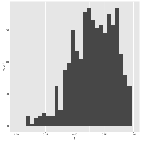
Looks like we’re in the right ballpark.

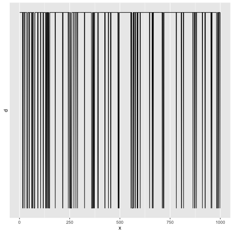
We can examine the traces of other elements of the program as well. Here’s the recorded distribution over component assignments, for example - note that the rightmost bar here corresponds to the leftmost component in the mixture:

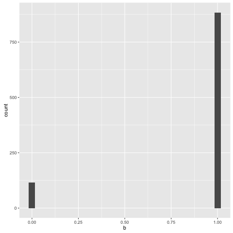
You can see that whenever we wandered into the rightmost component, we’d swiftly wind up jumping back out of it:

Comments

This is a fun take on probabilistic programming. In particular I find a few aspects of the whole setup to be pretty attractive:

We use a primitive, limited instruction set to parameterize both programs - via Free - and running programs - via Cofree. These off-the-shelf recursive types are used to wrap things up and provide most of our required control flow automatically. It’s easy to transparently add structure to embedded programs built in this way; for example, we can statically encode independence by replacing our ModelF a type with something like:

data InstructionF a = Coproduct (ModelF a) (Ap (ModelF a))

This can be hidden from the user so that we’re left with the same simple monadic syntax we presently enjoy, but we also get to take independence into account when performing inference, or any other structural interpretation for that matter.

When it comes to inference, the program representation is completely separate from whatever inference backend we choose to augment it with. We can deal with traces as first-class values that can be directly stored, inspected, manipulated, and so on. And everything is done in a typed and purely-functional framework. I’ve used dynamic typing functionality from Data.Dynamic to store values in execution traces here, but we could similarly just define a concrete Value type with the appropriate constructors for integers, doubles, bools, etc., and use that to store everything.

At the same time, this is a pretty early concept - doing inference efficiently in this setting is another matter, and there are a couple of computational and statistical issues here that need to be ironed out to make further progress.

The current way I’ve organized Markov chain generation and iteration is just woefully inefficient. Storing the history of each node on-site is needlessly costly and I’m sure results in a ton of unnecessary allocation. On a semantic level, it also ‘complects’ state and identity: why, after all, should a single execution trace know anything about traces that preceded it? Clearly this should be accumulated in another data structure. There is a lot of other low-hanging fruit around strictness and PRNG management as well.

From a more statistical angle, the present implementation does a poor job when it comes to perturbing execution traces. Some changes - such as improving the proposal mechanism for a given instruction - are easy to implement, and representing distributions as instructions indeed makes it easy to tailor local proposal distributions in a context-independent way. But another problem is that, by using a ‘blunt’ comonadic extend, we perturb an execution by perturbing every node in it. In general it’s better to make small perturbations rather than large ones to ensure a reasonable acceptance ratio, but to do that we’d need to perturb single nodes (or at least subsets of nodes) at a time.

There may be some inroads here via comonad transformers like StoreT or lenses that would allow us to zoom in on a particular node and perturb it, rather than perturbing everything at once. But my comonad-fu is not yet quite at the required level to evaluate this, so I’ll come back to that idea some other time.

I’m interested in playing with this concept some more in the future, though I’m not yet sure how much I expect it to be a tenable way to do inference at scale. If you’re interested in playing with it, I’ve dumped the code from this post into this gist.

Thanks to Niffe Hermansson and Fredrik Olsen for reviewing a draft of this post and providing helpful comments.