A Simple Embedded Probabilistic Programming Language

What does a dead-simple probabilistic programming language look like? The simplest thing I can imagine involves three components:

• A representation for probabilistic models.
• A way to simulate from those models (‘forward’ sampling).
• A way to sample from a conditional model (‘backward’ sampling).

Rob Zinkov wrote an article on this type of thing around a year ago, and Dan Roy recently gave a talk on the topic as well. In the spirit of unabashed unoriginality, I’ll give a sort of composite example of the two. Most of the material here comes directly from Dan’s talk; definitely check it out if you’re curious about this whole probabilistic programming mumbojumbo.

Let’s whip together a highly-structured, typed, embedded probabilistic programming language - the core of which will encompass a tiny amount of code.

Some preliminaries - note that you’ll need my simple little mwc-probability library handy for when it comes time to do sampling:

{-# LANGUAGE DeriveFunctor #-}
{-# LANGUAGE LambdaCase #-}

import Control.Monad
import Control.Monad.Free
import qualified System.Random.MWC.Probability as MWC

Representing Probabilistic Models

Step one is to represent the fundamental constructs found in probabilistic programs. These are abstract probability distributions; I like to call them models:

data ModelF r =
    BernoulliF Double (Bool -> r)
  | BetaF Double Double (Double -> r)
  deriving Functor

type Model = Free ModelF

Each foundational probability distribution we want to consider is represented as a constructor of the ModelF type. You can think of them as probabilistic instructions, in a sense. A Model itself is a program parameterized by this probabilistic instruction set.

In a more sophisticated implementation you’d probably want to add more primitives, but you can get pretty far with the beta and Bernoulli distributions alone. Here are some embedded language terms, only two of which correspond one-to-one with to the constructors themselves:

bernoulli :: Double -> Model Bool
bernoulli p = liftF (BernoulliF p id)

beta :: Double -> Double -> Model Double
beta a b = liftF (BetaF a b id)

uniform :: Model Double
uniform = beta 1 1

binomial :: Int -> Double -> Model Int
binomial n p = fmap count coins where
  count = length . filter id
  coins = replicateM n (bernoulli p)

betaBinomial :: Int -> Double -> Double -> Model Int
betaBinomial n a b = do
  p <- beta a b
  binomial n p

You can build a lot of other useful distributions by just starting from the beta and Bernoulli as well. And technically I guess the more foundational distributions to use here would be the Dirichlet and categorical, of which the beta and Bernoulli are special cases. But I digress. The point is that other distributions are easy to construct from a set of reliable primitives; you can check out the old lambda-naught paper by Park et al for more examples.

See how binomial and betaBinomial are defined? In the case of binomial we’re using the property that models have a functorial structure by just mapping a counting function over the result of a bunch of Bernoulli random variables. For betaBinomial we’re directly making use of our monadic structure, first describing a weight parameter via a beta distribution and then using it as an input to a binomial distribution.

Note in particular that we’ve expressed betaBinomial by binding a parameter model to a data model. This is a foundational pattern in Bayesian statistics; in the more usual lingo, the parameter model corresponds to the prior distribution, and the data model is the likelihood.

Forward-Mode Sampling

So we have our representation. Next up, we want to simulate from these models. Thus far they’re purely abstract, and don’t encode any information about probability or sampling or what have you. We have to ascribe that ourselves.

mwc-probability defines a monadic sampling-based probability distribution type called Prob, and we can use a basic recursion scheme on free monads to adapt our own model type to that:

toSampler :: Model a -> MWC.Prob IO a
toSampler = iterM $ \case
  BernoulliF p f -> MWC.bernoulli p >>= f
  BetaF a b f    -> MWC.beta a b >>= f

We can glue that around the relevant mwc-probability functionality to simulate from models directly:

simulate :: Model a -> IO a
simulate model = MWC.withSystemRandom . MWC.asGenIO $
  MWC.sample (toSampler model)

And this can be used with standard monadic combinators like replicateM to collect larger samples:

> replicateM 10 $ simulate (betaBinomial 10 1 4)
[5,7,1,4,4,1,1,0,4,2]

Reverse-Mode Sampling

Now. Here we want to condition our model on some observations and then recover the conditional distribution over its internal parameters.

This part - inference - is what makes probabilistic programming hard, and doing it really well remains an unsolved problem. One of the neat theoretical results in this space due to Ackerman, Freer, and Roy is that in the general case the problem is actually unsolvable, in that one can encode as a probabilistic program a conditional distribution that computes the halting problem. Similarly, in general it’s impossible to do this sort of thing efficiently even for computable conditional distributions. Consider the case of a program that returns the hash of a random n-long binary string, and then try to infer the distribution over strings given some hashes, for example. This is never going to be a tractable problem.

For now let’s use a simple rejection sampler to encode a conditional distribution. We’ll require some observations, a proposal distribution, and the model that we want to invert:

invert :: (Monad m, Eq b) => m a -> (a -> m b) -> [b] -> m a
invert proposal model observed = loop where
  loop = do
    parameters <- proposal
    generated  <- replicateM (length observed) (model parameters)
    if   generated == observed
    then return parameters
    else loop

Let’s use it to compute the posterior or inverse model of an (apparently) biased coin, given a few observations. We’ll just use a uniform distribution as our proposal:

posterior :: Model Double
posterior = invert [True, True, False, True] uniform bernoulli

Let’s grab some samples from the posterior distribution:

> replicateM 1000 (simulate posterior)

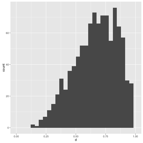
The central tendency of the posterior floats about 0.75, which is what we’d expect, given our observations. This has been inferred from only four points; let’s try adding a few more. But before we do that, note that the present way the rejection sampling algorithm works is:

• Propose a parameter value according to the supplied proposal distribution.
• Generate a sample from the model, of equal size to the supplied observations.
• Compare the collected sample to the supplied observations. If they’re equal, then return the proposed parameter value. Otherwise start over.

Rejection sampling isn’t exactly efficient in nontrivial settings anyway, but it’s supremely inefficient for our present case. The random variables we’re interested in are exchangeable, so what we’re concerned about is the total number of True or False values observed - not any specific order they appear in.

We can add an ‘assistance’ function to the rejection sampler to help us out in this case:

invertWithAssistance
  :: (Monad m, Eq c) => ([a] -> c) -> m b -> (b -> m a) -> [a] -> m b
invertWithAssistance assister proposal model observed = loop where
  loop = do
    parameters <- proposal
    generated  <- replicateM (length observed) (model parameters)
    if   assister generated == assister observed
    then return parameters
    else loop

The assister summarizes both our observations and collected sample to ensure they’re efficiently comparable. In our situation, we can use a simple counting function to tally up the number of True values we observe:

count :: [Bool] -> Int
count = length . filter id

Now let’s create another posterior by conditioning on a few more observations:

posterior0 :: Model Double
posterior0 = invertWithAssitance count uniform bernoulli obs where
  obs =
    [True, True, True, False, True, True, False, True, True, True, True, False]

and collect another thousand samples from it. This would likely take an annoying amount of time without the use of our count function for assistance above:

> replicateM 1000 (simulate posterior0)

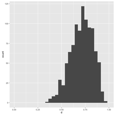
Note that with more information to condition on, we get a more informative posterior.

Conclusion

This is a really basic formulation - too basic to be useful in any meaningful way - but it illustrates some of the most important concepts in probabilistic programming. Representation, simulation, and inference.

I think it’s also particularly nice to do this in Haskell, rather than something like Python (which Dan used in his talk) - it provides us with a lot of extensible structure in a familiar framework for language hacking. It sort of demands you’re a fan of all these higher-kinded types and structured recursions and all that, but if you’re reading this blog then you’re probably in that camp anyway.

I’ll probably write a few more little articles like this over time. There are a ton of improvements that we can make to this basic setup - encoding independence, sampling via MCMC, etc. - and it might be fun to grow everything out piece by piece.

I’ve dropped the code from this post into this gist.