Recursive Stochastic Processes
01 Mar 2017Last week Dan Peebles asked me on Twitter if I knew of any writing on the use of recursion schemes for expressing stochastic processes or other probability distributions. And I don’t! So I’ll write some of what I do know myself.
There are a number of popular statistical models or stochastic processes that have an overtly recursive structure, and when one has some recursive structure lying around, the elegant way to represent it is by way of a recursion scheme. In the case of stochastic processes, this typically boils down to using an anamorphism to drive things. Or, if you actually want to be able to observe the thing (note: you do), an apomorphism.
By representing a stochastic process in this way one can really isolate the probabilistic phenomena involved in it. One bundles up the essence of a process in a coalgebra, and then drives it via some appropriate recursion scheme.
Let’s take a look at three stochastic processes and examine their probabilistic and recursive structures.
Foundations
To start, I’m going to construct a simple embedded language in the spirit of the ones used in my simple probabilistic programming and comonadic inference posts. Check those posts out if this stuff looks too unfamiliar. Here’s a preamble that constitutes the skeleton of the code we’ll be working with.
{-# LANGUAGE DeriveFunctor #-}
{-# LANGUAGE FlexibleContexts #-}
{-# LANGUAGE LambdaCase #-}
{-# LANGUAGE RankNTypes #-}
{-# LANGUAGE TypeFamilies #-}

import Control.Monad
import Control.Monad.Free
import qualified Control.Monad.Trans.Free as TF
import Data.Functor.Foldable
import Data.Random (RVar, sample)
import qualified Data.Random.Distribution.Bernoulli as RF
import qualified Data.Random.Distribution.Beta as RF
import qualified Data.Random.Distribution.Normal as RF

-- probabilistic instruction set, program definitions

data ModelF a r =
    BernoulliF Double (Bool -> r)
  | GaussianF Double Double (Double -> r)
  | BetaF Double Double (Double -> r)
  | DiracF a
  deriving Functor

type Program a = Free (ModelF a)

type Model b = forall a. Program a b

type Terminating a = Program a a

-- core language terms

bernoulli :: Double -> Model Bool
bernoulli p = liftF (BernoulliF vp id) where
  vp
    | p < 0 = 0
    | p > 1 = 1
    | otherwise = p

gaussian :: Double -> Double -> Model Double
gaussian m s
  | s <= 0    = error "gaussian: variance out of bounds"
  | otherwise = liftF (GaussianF m s id)

beta :: Double -> Double -> Model Double
beta a b
  | a <= 0 || b <= 0 = error "beta: parameter out of bounds"
  | otherwise        = liftF (BetaF a b id)

dirac :: a -> Program a b
dirac x = liftF (DiracF x)

-- interpreter

rvar :: Program a a -> RVar a
rvar = iterM $ \case
  BernoulliF p f  -> RF.bernoulli p >>= f
  GaussianF m s f -> RF.normal m s >>= f
  BetaF a b f     -> RF.beta a b >>= f
  DiracF x        -> return x

-- utilities

free :: Functor f => Fix f -> Free f a
free = cata Free

affine :: Num a => a -> a -> a -> a
affine translation scale = (+ translation) . (* scale)
Just as a quick review, we’ve got:
- A probabilistic instruction set defined by ‘ModelF’. Each constructor represents a foundational probability distribution that we can use in our embedded programs.
- Three types corresponding to probabilistic programs. The ‘Program’ type simply wraps our instruction set up in a naïve free monad. The ‘Model’ type denotes probabilistic programs that may not necessarily terminate (in some weak sense), while the ‘Terminating’ type denotes probabilistic programs that terminate (ditto).
- A bunch of embedded language terms. These are just probability distributions; here we’ll manage with the Bernouli, Gaussian, and beta distributions. We also have a ‘dirac’ term for constructing a Dirac distribution at a point.
- A single interpeter ‘rvar’ that interprets a probabilistic program into a random variable (where the ‘RVar’ type is provided by random-fu). Typically I use mwc-probability for this but random-fu is quite nice. When a program has been interpreted into a random variable we can use ‘sample’ to sample from it.
So: we can write simple probabilistic programs in standard monadic fashion, like so:
betaBernoulli :: Double -> Double -> Model Bool
betaBernoulli a b = do
  p <- beta a b
  bernoulli p
and then interpret them as needed:
> replicateM 10 (sample (rvar (betaBernoulli 1 8)))
[False,False,False,False,False,False,False,True,True,False]
The Geometric Distribution
The geometric distribution is not a stochastic process per se, but it can be represented by one. If we repeatedly flip a coin and then count the number of flips until the first head, and then consider the probability distribution over that count, voilà. That’s the geometric distribution. You might see a head right away, or you might be infinitely unlucky and never see a head. So the distribution is supported over the entirety of the natural numbers.
For illustration, we can encode the coin flipping process in a straightforward recursive manner:
simpleGeometric :: Double -> Terminating Int
simpleGeometric p = loop 1 where
  loop n = do
    accept <- bernoulli p
    if   accept
    then dirac n
    else loop (n + 1)
We start flipping Bernoulli-distributed coins, and if we observe a head we stop and return the number of coins flipped thus far. Otherwise we keep flipping.
The underlying probabilistic phenomena here are the Bernoulli draw, which determines if we’ll terminate, and the dependent Dirac return, which will wrap a terminating value in a point mass. The recursive procedure itself has the pattern of:
- If some condition is met, abort the recursion and return a value.
- Otherwise, keep recursing.
This pattern describes an apomorphism, and the recursion-schemes type signature of ‘apo’ is:
apo :: Corecursive t => (a -> Base t (Either t a)) -> a -> t
It takes a coalgebra that returns an ‘Either’ value wrapped up in a base functor, and uses that coalgebra to drive the recursion. A ‘Left’-returned value halts the recursion, while a ‘Right’-returned value keeps it going.
Don’t be put off by the type of the coalgebra if you’re unfamiliar with apomorphisms - its bark is worse than its bite. Check out my older post on apomorphisms for a brief introduction to them.
With reference to the ‘apo’ type signature, The main thing to choose here is the recursive type that we’ll use to wrap up the ‘ModelF’ base functor. ‘Fix’ might be conceivably simpler to start, so I’ll begin with that. The coalgebra defining the model looks like this:
geoCoalg p n = BernoulliF p (\accept ->
  if   accept
  then Left (Fix (DiracF n))
  else Right (n + 1))
Then given the coalgebra, we can just wrap it up in ‘apo’ to represent the geometric distribution.
geometric :: Double -> Terminating Int
geometric p = free (apo (geoCoalg p) 1)
Since the geometric distribution (weakly) terminates, the program has return type ‘Terminating Int’.
Since we’ve encoded the coalgebra using ‘Fix’, we have to explicitly convert to ‘Free’ via the ‘free’ utility function I defined in the preamble. Recent versions of recursion-schemes have added a ‘Corecursive’ instance for ‘Free’, though, so the superior alternative is to just use that:
geometric :: Double -> Terminating Int
geometric p = apo coalg 1 where
  coalg n = TF.Free (BernoulliF p (\accept ->
    if   accept
    then Left (dirac n)
    else Right (n + 1)))
The point of all this is that we can isolate the core probabilistic phenomena of the recursive process by factoring it out into a coalgebra. The recursion itself takes the form of an apomorphism, which knows nothing about probability or flipping coins or what have you - it just knows how to recurse, or stop.
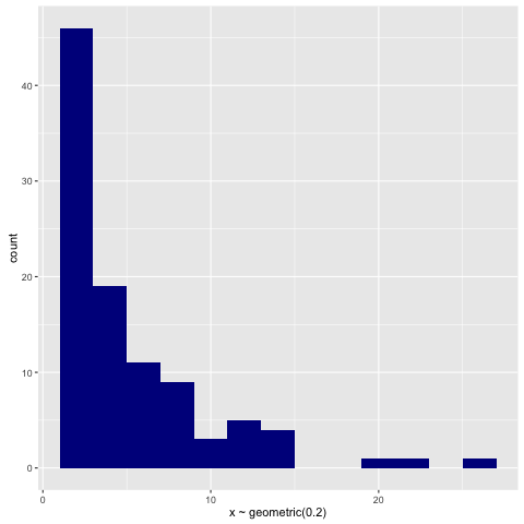
For illustration, here’s a histogram of samples drawn from the geometric via:
> replicateM 100 (sample (rvar (geometric 0.2)))
An Autoregressive Process
Autoregressive (AR) processes simply use a previous epoch’s output as the current epoch’s input; the number of previous epochs used as input on any given epoch is called the order of the process. An AR(1) process looks like this, for example:
\[y_t = \alpha + \beta y_{t - 1} + \epsilon_t\]Here \(\epsilon_t\) are independent and identically-distributed random variables that follow some error distribution. In other words, in this model the value \(\alpha + \beta y_{t - 1}\) follows some probability distribution given the last epoch’s output \(y_{t - 1}\) and some parameters \(\alpha\) and \(\beta\).
An autoregressive process doesn’t have any notion of termination built into it, so the purest way to represent one is via an anamorphism. We’ll focus on AR(1) processes in this example:
ar1 :: Double -> Double -> Double -> Double -> Model Double
ar1 a b s = ana coalg where
  coalg x = TF.Free (GaussianF (affine a b x) s (affine a b))
Each epoch is just a Gaussian-distributed affine transformation of the previous epochs’s output. But the problem with using an anamorphism here is that it will just shoot off to infinity, recursing endlessly. This doesn’t do us a ton of good if we want to actually observe the process, so if we want to do that we’ll need to bake in our own conditions for termination. Again we’ll rely on an apomorphism for this; we can just specify how many periods we want to observe the process for, and stop recursing as soon as we exceed that.
There are two ways to do this. We can either get a view of the process at \(n\) periods in the future, or we can get a view of the process over \(n\) periods in the future. I’ll write both, for illustration. The coalgebra for the first is simpler, and looks like:
arCoalg (n, x) = TF.Free (GaussianF (affine a b x) s (\y ->
    if   n <= 0
    then Left (dirac x)
    else Right (pred m, y)))
The coalgebra is saying:
- Given \(x\), let \(z\) have a Gaussian distribution with mean \(\alpha + \beta x\) and standard deviation \(s\).
- If we’re on the last epoch, return \(x\) as a Dirac point mass.
- Otherwise, continue recursing with \(z\) as input to the next epoch.
Now, to observe the process over the next \(n\) periods we can just collect the observations we’ve seen so far in a list. An implementation of the process, apomorphism and all, looks like this:
ar :: Int -> Double -> Double -> Double -> Double -> Terminating [Double]
ar n a b s origin = apo coalg (n, [origin]) where
  coalg (epochs, history@(x:_)) =
    TF.Free (GaussianF (affine a b x) s (\y ->
      if   epochs <= 0
      then Left (dirac (reverse history))
      else Right (pred epochs, y:history)))
(Note that I’m deliberately not handling the error condition here so as to focus on the essence of the coalgebra.)
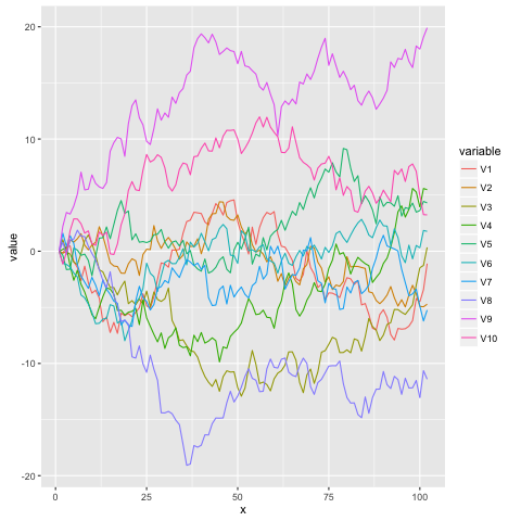
We can generate some traces for it in the standard way. Here’s how we’d sample a 100-long trace from an AR(1) process originating at 0 with \(\alpha = 0\), \(\beta = 1\), and \(s = 1\):
> sample (rvar (ar 100 0 1 1 0))
and here’s a visualization of 10 of those traces:
The Stick-Breaking Process
The stick breaking process is one of any number of whimsical stochastic processes used as prior distributions in nonparametric Bayesian models. The idea here is that we want to take a stick and endlessly break it into smaller and smaller pieces. Every time we break a stick, we recursively take the rest of the stick and break it again, ad infinitum.
Again, if we wanted to represent this endless process very faithfully, we’d use an anamorphism to drive it. But in practice we’re going to only want to break a stick some finite number of times, so we’ll follow the same pattern as the AR process and use an apomorphism to do that:
sbp :: Int -> Double -> Terminating [Double]
sbp n a = apo coalg (n, 1, []) where
  coalg (epochs, stick, sticks) = TF.Free (BetaF 1 a (\p ->
    if   epochs <= 0
    then Left (dirac (reverse (stick : sticks)))
    else Right (pred epochs, (1 - p) * stick, (p * stick):sticks)))
The coalgebra that defines the process says the following:
- Let the location \(p\) of the break on the next (normalized) stick be beta\((1, \alpha)\)-distributed.
- If we’re on the last epoch, return all the pieces of the stick that we broke as a Dirac point mass.
- Otherwise, break the stick again and recurse.
Here’s a plot of five separate draws from a stick breaking process with \(\alpha = 0.2\), each one observed for five breaks. Note that each draw encodes a categorical distribution over the set \(\{1, \ldots, 6\}\); the stick breaking process is a ‘distribution over distributions’ in that sense:
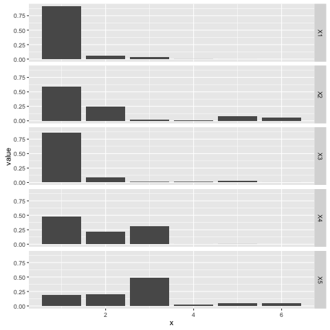
The stick breaking process is useful for developing mixture models with an unknown number of components, for example. The \(\alpha\) parameter can be tweaked to concentrate or disperse probability mass as needed.
Conclusion
This seems like enough for now. I’d be interested in exploring other models generated by recursive processes just to see how they can be encoded, exactly. Basically all of Bayesian nonparametrics is based on using recursive processses as prior distributions, so the Dirichlet process, Chinese Restaurant Process, Indian Buffet Process, etc. should work beautifully in this setting.
Fun fact: back in 2011 before neural networks deep learning had taken over
machine learning, Bayesian nonparametrics was probably the hottest research
area in town. I used to joke that I’d create a new prior called the Malaysian
Takeaway Process for some esoteric nonparametric model and thus achieve machine
learning fame, but never did get around to that.
Addendum
I got a question about how I produce these plots. And the answer is the only sane way when it comes to visualization in Haskell: dump the output to disk and plot it with something else. I use R for most of my interactive/exploratory data science-fiddling, as well as for visualization. Python with matplotlib is obviously a good choice too.
Here’s how I made the autoregressive process plot, for example. First, I just produced the actual samples in GHCi:
> samples <- replicateM 10 (sample (rvar (ar 100 0 1 1 0)))
Then I wrote them to disk:
> let render handle = hPutStrLn handle . filter (`notElem` "[]") . show
> withFile "trace.dat" WriteMode (\handle -> mapM_ (render handle) samples)
The following R script will then get you the plot:
require(ggplot2)
require(reshape2)

raw = read.csv('trace.dat', header = F)

d = data.frame(t(raw), x = seq_along(raw))
m = melt(d, id.vars = 'x')

ggplot(m, aes(x, value, colour = variable)) + geom_line()
I used ggplot2 for the other plots as well; check out the ggplot2
functions geom_histogram, geom_bar, and facet_grid in particular.