Recursive Stochastic Processes

Last week Dan Peebles asked me on Twitter if I knew of any writing on the use of recursion schemes for expressing stochastic processes or other probability distributions. And I don’t! So I’ll write some of what I do know myself.

There are a number of popular statistical models or stochastic processes that have an overtly recursive structure, and when one has some recursive structure lying around, the elegant way to represent it is by way of a recursion scheme. In the case of stochastic processes, this typically boils down to using an anamorphism to drive things. Or, if you actually want to be able to observe the thing (note: you do), an apomorphism.

By representing a stochastic process in this way one can really isolate the probabilistic phenomena involved in it. One bundles up the essence of a process in a coalgebra, and then drives it via some appropriate recursion scheme.

Let’s take a look at three stochastic processes and examine their probabilistic and recursive structures.

Foundations

To start, I’m going to construct a simple embedded language in the spirit of the ones used in my simple probabilistic programming and comonadic inference posts. Check those posts out if this stuff looks too unfamiliar. Here’s a preamble that constitutes the skeleton of the code we’ll be working with.

{-# LANGUAGE DeriveFunctor #-}
{-# LANGUAGE FlexibleContexts #-}
{-# LANGUAGE LambdaCase #-}
{-# LANGUAGE RankNTypes #-}
{-# LANGUAGE TypeFamilies #-}

import Control.Monad
import Control.Monad.Free
import qualified Control.Monad.Trans.Free as TF
import Data.Functor.Foldable
import Data.Random (RVar, sample)
import qualified Data.Random.Distribution.Bernoulli as RF
import qualified Data.Random.Distribution.Beta as RF
import qualified Data.Random.Distribution.Normal as RF

-- probabilistic instruction set, program definitions

data ModelF a r =
    BernoulliF Double (Bool -> r)
  | GaussianF Double Double (Double -> r)
  | BetaF Double Double (Double -> r)
  | DiracF a
  deriving Functor

type Program a = Free (ModelF a)

type Model b = forall a. Program a b

type Terminating a = Program a a

-- core language terms

bernoulli :: Double -> Model Bool
bernoulli p = liftF (BernoulliF vp id) where
  vp
    | p < 0 = 0
    | p > 1 = 1
    | otherwise = p

gaussian :: Double -> Double -> Model Double
gaussian m s
  | s <= 0    = error "gaussian: variance out of bounds"
  | otherwise = liftF (GaussianF m s id)

beta :: Double -> Double -> Model Double
beta a b
  | a <= 0 || b <= 0 = error "beta: parameter out of bounds"
  | otherwise        = liftF (BetaF a b id)

dirac :: a -> Program a b
dirac x = liftF (DiracF x)

-- interpreter

rvar :: Program a a -> RVar a
rvar = iterM $ \case
  BernoulliF p f  -> RF.bernoulli p >>= f
  GaussianF m s f -> RF.normal m s >>= f
  BetaF a b f     -> RF.beta a b >>= f
  DiracF x        -> return x

-- utilities

free :: Functor f => Fix f -> Free f a
free = cata Free

affine :: Num a => a -> a -> a -> a
affine translation scale = (+ translation) . (* scale)

Just as a quick review, we’ve got:

• A probabilistic instruction set defined by ‘ModelF’. Each constructor represents a foundational probability distribution that we can use in our embedded programs.
• Three types corresponding to probabilistic programs. The ‘Program’ type simply wraps our instruction set up in a naïve free monad. The ‘Model’ type denotes probabilistic programs that may not necessarily terminate (in some weak sense), while the ‘Terminating’ type denotes probabilistic programs that terminate (ditto).
• A bunch of embedded language terms. These are just probability distributions; here we’ll manage with the Bernouli, Gaussian, and beta distributions. We also have a ‘dirac’ term for constructing a Dirac distribution at a point.
• A single interpeter ‘rvar’ that interprets a probabilistic program into a random variable (where the ‘RVar’ type is provided by random-fu). Typically I use mwc-probability for this but random-fu is quite nice. When a program has been interpreted into a random variable we can use ‘sample’ to sample from it.

So: we can write simple probabilistic programs in standard monadic fashion, like so:

betaBernoulli :: Double -> Double -> Model Bool
betaBernoulli a b = do
  p <- beta a b
  bernoulli p

and then interpret them as needed:

> replicateM 10 (sample (rvar (betaBernoulli 1 8)))
[False,False,False,False,False,False,False,True,True,False]

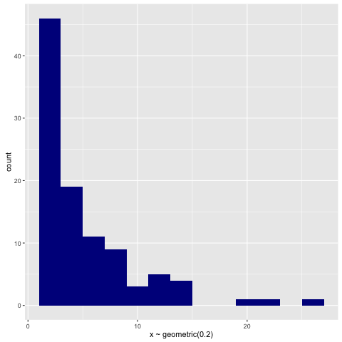
The Geometric Distribution

The geometric distribution is not a stochastic process per se, but it can be represented by one. If we repeatedly flip a coin and then count the number of flips until the first head, and then consider the probability distribution over that count, voilà. That’s the geometric distribution. You might see a head right away, or you might be infinitely unlucky and never see a head. So the distribution is supported over the entirety of the natural numbers.

For illustration, we can encode the coin flipping process in a straightforward recursive manner:

simpleGeometric :: Double -> Terminating Int
simpleGeometric p = loop 1 where
  loop n = do
    accept <- bernoulli p
    if   accept
    then dirac n
    else loop (n + 1)

We start flipping Bernoulli-distributed coins, and if we observe a head we stop and return the number of coins flipped thus far. Otherwise we keep flipping.

The underlying probabilistic phenomena here are the Bernoulli draw, which determines if we’ll terminate, and the dependent Dirac return, which will wrap a terminating value in a point mass. The recursive procedure itself has the pattern of:

• If some condition is met, abort the recursion and return a value.
• Otherwise, keep recursing.

This pattern describes an apomorphism, and the recursion-schemes type signature of ‘apo’ is:

apo :: Corecursive t => (a -> Base t (Either t a)) -> a -> t

It takes a coalgebra that returns an ‘Either’ value wrapped up in a base functor, and uses that coalgebra to drive the recursion. A ‘Left’-returned value halts the recursion, while a ‘Right’-returned value keeps it going.

Don’t be put off by the type of the coalgebra if you’re unfamiliar with apomorphisms - its bark is worse than its bite. Check out my older post on apomorphisms for a brief introduction to them.

With reference to the ‘apo’ type signature, The main thing to choose here is the recursive type that we’ll use to wrap up the ‘ModelF’ base functor. ‘Fix’ might be conceivably simpler to start, so I’ll begin with that. The coalgebra defining the model looks like this:

geoCoalg p n = BernoulliF p (\accept ->
  if   accept
  then Left (Fix (DiracF n))
  else Right (n + 1))

Then given the coalgebra, we can just wrap it up in ‘apo’ to represent the geometric distribution.

geometric :: Double -> Terminating Int
geometric p = free (apo (geoCoalg p) 1)

Since the geometric distribution (weakly) terminates, the program has return type ‘Terminating Int’.

Since we’ve encoded the coalgebra using ‘Fix’, we have to explicitly convert to ‘Free’ via the ‘free’ utility function I defined in the preamble. Recent versions of recursion-schemes have added a ‘Corecursive’ instance for ‘Free’, though, so the superior alternative is to just use that:

geometric :: Double -> Terminating Int
geometric p = apo coalg 1 where
  coalg n = TF.Free (BernoulliF p (\accept ->
    if   accept
    then Left (dirac n)
    else Right (n + 1)))

The point of all this is that we can isolate the core probabilistic phenomena of the recursive process by factoring it out into a coalgebra. The recursion itself takes the form of an apomorphism, which knows nothing about probability or flipping coins or what have you - it just knows how to recurse, or stop.

For illustration, here’s a histogram of samples drawn from the geometric via:

> replicateM 100 (sample (rvar (geometric 0.2)))

An Autoregressive Process

Autoregressive (AR) processes simply use a previous epoch’s output as the current epoch’s input; the number of previous epochs used as input on any given epoch is called the order of the process. An AR(1) process looks like this, for example:

Here \(\epsilon_t\) are independent and identically-distributed random variables that follow some error distribution. In other words, in this model the value \(\alpha + \beta y_{t - 1}\) follows some probability distribution given the last epoch’s output \(y_{t - 1}\) and some parameters \(\alpha\) and \(\beta\).

An autoregressive process doesn’t have any notion of termination built into it, so the purest way to represent one is via an anamorphism. We’ll focus on AR(1) processes in this example:

ar1 :: Double -> Double -> Double -> Double -> Model Double
ar1 a b s = ana coalg where
  coalg x = TF.Free (GaussianF (affine a b x) s (affine a b))

Each epoch is just a Gaussian-distributed affine transformation of the previous epochs’s output. But the problem with using an anamorphism here is that it will just shoot off to infinity, recursing endlessly. This doesn’t do us a ton of good if we want to actually observe the process, so if we want to do that we’ll need to bake in our own conditions for termination. Again we’ll rely on an apomorphism for this; we can just specify how many periods we want to observe the process for, and stop recursing as soon as we exceed that.

There are two ways to do this. We can either get a view of the process at \(n\) periods in the future, or we can get a view of the process over \(n\) periods in the future. I’ll write both, for illustration. The coalgebra for the first is simpler, and looks like:

arCoalg (n, x) = TF.Free (GaussianF (affine a b x) s (\y ->
    if   n <= 0
    then Left (dirac x)
    else Right (pred m, y)))

The coalgebra is saying:

• Given \(x\), let \(z\) have a Gaussian distribution with mean \(\alpha + \beta x\) and standard deviation \(s\).
• If we’re on the last epoch, return \(x\) as a Dirac point mass.
• Otherwise, continue recursing with \(z\) as input to the next epoch.

Now, to observe the process over the next \(n\) periods we can just collect the observations we’ve seen so far in a list. An implementation of the process, apomorphism and all, looks like this:

ar :: Int -> Double -> Double -> Double -> Double -> Terminating [Double]
ar n a b s origin = apo coalg (n, [origin]) where
  coalg (epochs, history@(x:_)) =
    TF.Free (GaussianF (affine a b x) s (\y ->
      if   epochs <= 0
      then Left (dirac (reverse history))
      else Right (pred epochs, y:history)))

(Note that I’m deliberately not handling the error condition here so as to focus on the essence of the coalgebra.)

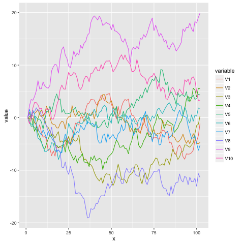
We can generate some traces for it in the standard way. Here’s how we’d sample a 100-long trace from an AR(1) process originating at 0 with \(\alpha = 0\), \(\beta = 1\), and \(s = 1\):

> sample (rvar (ar 100 0 1 1 0))

and here’s a visualization of 10 of those traces:

The Stick-Breaking Process

The stick breaking process is one of any number of whimsical stochastic processes used as prior distributions in nonparametric Bayesian models. The idea here is that we want to take a stick and endlessly break it into smaller and smaller pieces. Every time we break a stick, we recursively take the rest of the stick and break it again, ad infinitum.

Again, if we wanted to represent this endless process very faithfully, we’d use an anamorphism to drive it. But in practice we’re going to only want to break a stick some finite number of times, so we’ll follow the same pattern as the AR process and use an apomorphism to do that:

sbp :: Int -> Double -> Terminating [Double]
sbp n a = apo coalg (n, 1, []) where
  coalg (epochs, stick, sticks) = TF.Free (BetaF 1 a (\p ->
    if   epochs <= 0
    then Left (dirac (reverse (stick : sticks)))
    else Right (pred epochs, (1 - p) * stick, (p * stick):sticks)))

The coalgebra that defines the process says the following:

• Let the location \(p\) of the break on the next (normalized) stick be beta\((1, \alpha)\)-distributed.
• If we’re on the last epoch, return all the pieces of the stick that we broke as a Dirac point mass.
• Otherwise, break the stick again and recurse.

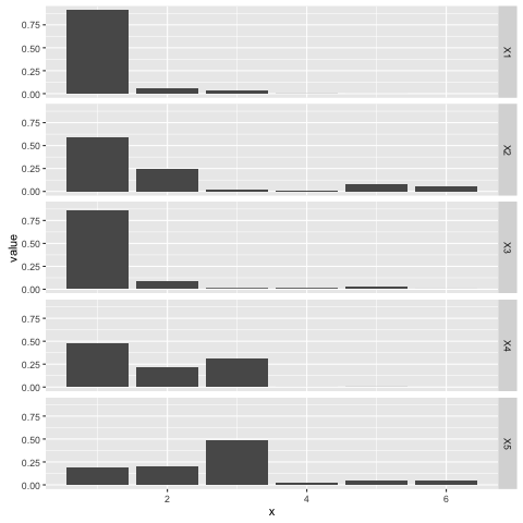
Here’s a plot of five separate draws from a stick breaking process with \(\alpha = 0.2\), each one observed for five breaks. Note that each draw encodes a categorical distribution over the set \(\{1, \ldots, 6\}\); the stick breaking process is a ‘distribution over distributions’ in that sense:

The stick breaking process is useful for developing mixture models with an unknown number of components, for example. The \(\alpha\) parameter can be tweaked to concentrate or disperse probability mass as needed.

Conclusion

This seems like enough for now. I’d be interested in exploring other models generated by recursive processes just to see how they can be encoded, exactly. Basically all of Bayesian nonparametrics is based on using recursive processses as prior distributions, so the Dirichlet process, Chinese Restaurant Process, Indian Buffet Process, etc. should work beautifully in this setting.

Fun fact: back in 2011 before neural networks deep learning had taken over machine learning, Bayesian nonparametrics was probably the hottest research area in town. I used to joke that I’d create a new prior called the Malaysian Takeaway Process for some esoteric nonparametric model and thus achieve machine learning fame, but never did get around to that.

Addendum

I got a question about how I produce these plots. And the answer is the only sane way when it comes to visualization in Haskell: dump the output to disk and plot it with something else. I use R for most of my interactive/exploratory data science-fiddling, as well as for visualization. Python with matplotlib is obviously a good choice too.

Here’s how I made the autoregressive process plot, for example. First, I just produced the actual samples in GHCi:

> samples <- replicateM 10 (sample (rvar (ar 100 0 1 1 0)))

Then I wrote them to disk:

> let render handle = hPutStrLn handle . filter (`notElem` "[]") . show
> withFile "trace.dat" WriteMode (\handle -> mapM_ (render handle) samples)

The following R script will then get you the plot:

require(ggplot2)
require(reshape2)

raw = read.csv('trace.dat', header = F)

d = data.frame(t(raw), x = seq_along(raw))
m = melt(d, id.vars = 'x')

ggplot(m, aes(x, value, colour = variable)) + geom_line()

I used ggplot2 for the other plots as well; check out the ggplot2 functions geom_histogram, geom_bar, and facet_grid in particular.

The Applicative Structure of the Giry Monad

In my last two posts about the Giry monad I derived the thing from its categorical and measure-theoretic foundations. I kind of thought that those posts wouldn’t be of much interest to people but they turned out to be a hit. I clearly can’t tell what the internet likes.

Anyway, something I left out was the theoretical foundation of the Giry monad’s Applicative instance, which seemed a bit odd. I also pointed out that applicativeness in the context of probability implies independence between probability measures.

In this article I’m going to look at each of these issues. After playing around with the foundations, it looks like the applicative instance for the Giry monad can be put on a sound footing in terms of the standard measure-theoretic concept of product measure. Also, it turns out that the claim I made of applicativeness \(\implies\) independence is somewhat ill-posed. But, using the shiny new intuition we’ll glean from a better understanding of the applicative structure, we can put that on a solid footing too.

So let’s look at both of these things and see what’s up.

Monoidal Functors

The foundational categorical concept behind applicative functors is the monoidal functor, which is a functor between monoidal categories that preserves monoidal structure.

Formally: for monoidal categories \((C, \otimes, I)\) and \((D, \oplus, J)\), a monoidal functor \(F : C \to D\) is a functor and associated natural transformations \(\phi : F(A) \oplus F(B) \to F(A \otimes B)\) and \(i : J \to F(I)\) that satisfy some coherence conditions that I won’t mention here. Notably, if \(\phi\) and \(i\) are isomorphisms (i.e. are invertible) then \(F\) is called a strong monoidal functor. Otherwise it’s called lax. Applicative functors in particular are lax monoidal functors.

This can be made much clearer for endofunctors on a monoidal category \((C, \otimes, I)\). Then you only have \(F : C \to C\) and \(\phi : F(A) \otimes F(B) \to F(A \otimes B)\) to worry about. If we sub in the Giry monad \(\mathcal{P}\) from the last couple of posts, we’d want \(\mathcal{P} : \textbf{Meas} \to \textbf{Meas}\) and \(\phi : \mathcal{P}(M) \otimes \mathcal{P}(N) \to \mathcal{P}(M \otimes N)\).

Does the category of measurable spaces \(\textbf{Meas}\) have a monoidal structure? Yup. Take measurable spaces \(M = (X, \mathcal{X})\) and \(N = (Y, \mathcal{Y})\). From the Giry monad derivation we already have that the monoidal identity \(i : M \to \mathcal{P}(M)\) corresponds to a Dirac measure at a point, so that’s well and good. And we can define the tensor product \(\otimes\) between \(M\) and \(N\) as follows: let \(X \times Y\) be the standard Cartesian product on \(X\) and \(Y\) and let \(\mathcal{X} \otimes \mathcal{Y}\) be the smallest \(\sigma\)-algebra generated by the Cartesian product \(A \times B\) of measurable sets \(A \in \mathcal{X}\) and \(B \in \mathcal{Y}\). Then \((X \times Y, \mathcal{X} \otimes \mathcal{Y})\) is a measurable space, and so \((\textbf{Meas}, \otimes, i)\) is monoidal.

Recall that \(\mathcal{P}(M)\) and \(\mathcal{P}(N)\) - the space of measures over \(M\) and \(N\) respectively - are themselves objects in \(\textbf{Meas}\). So, clearly \(\mathcal{P}(M) \otimes \mathcal{P}(N)\) is a measurable space, and if \(\mathcal{P}\) is monoidal then there must exist a natural transformation that can take us from there to \(\mathcal{P}(M \otimes N)\). This is the space of measures over the product \(M \otimes N\).

So the question is: does \(\mathcal{P}\) have the required monoidal structure?

Yes. It must, since \(\mathcal{P}\) is a monad, and any monad can generate the required natural transformation. Let \(\mu\) be the monadic ‘join’ operator \(\mathcal{P}^2 \to \mathcal{P}\) and \(\eta\) be the monadic identity \(I \to \mathcal{P}\). We have, evaluating right-to-left:

Using \(\gg\!\!=\) makes this much easier to read:

or in code, just:

phi :: Monad m => (m a, m b) -> m (a, b)
phi (m, n) = liftM2 (,) m n

So with that we have that \((\mathcal{P}, \phi, i)\) is a (lax) monoidal functor. And you can glean a monad-generated applicative operator from that immediately (this leads to the function called ‘ap’ in Control.Monad):

ap :: Monad m => m (a -> b) -> m a -> m b
ap f x = fmap (\(g, z) -> g z) (phi f x)

(Note: I won’t refer to \(\mu\) as the join operator from this point out in order to free it up for denoting measures.)

Probabilistic Interpretations

Product Measure

The correct probabilistic interpretation here is that \(\phi\) takes a pair of probability measures to the product measure over the appropriate product space. For probability measures \(\mu\) and \(\nu\) on measurable spaces \(M\) and \(N\) respectively, the product measure is the (unique) measure \(\mu \times \nu\) on \(M \otimes N\) such that:

for \(A \times B\) a measurable set in \(M \otimes N\).

Going through the monoidal functor route seems to put the notion of the Giry applicative instance on a more firm measure-theoretic foundation. Instead of considering the following from the Giry monad foundations article:

which is defined in terms of the dubious space of measures over measurable functions \(M \to N\), we can better view things using the monoidal structure-preserving natural transformation \(\phi\). For measures \(\mu\) and \(\nu\) on \((X, \mathcal{X})\) and \((Y, \mathcal{Y})\) respectively, we have:

and then for \(g : Z \to X \otimes Y\) we can use the functor structure of \(\mathcal{P}\) to do:

which corresponds to a standard applicative expression g <$> mu <*> nu. I suspect there’s then some sort of Yoneda argument or something that makes currying and partial function application acceptable.

Independence

Now. What does this have to say about independence?

In particular, it’s too fast and loose to claim measures can be ‘independent’ at all. Independence is a property of measurable sets, measurable functions, and \(\sigma\)-algebras. Not of measures! But there is a really useful connection, so let’s illustrate that.

First, let’s define independence formally as follows. Take a probability space \((X, \mathcal{X}, \mathbb{P})\). Then any measurable sets \(A\) and \(B\) in \(\mathcal{X}\) are independent if

That’s the simplest notion.

Next, consider two sub-\(\sigma\)-algebras \(\mathcal{A}\) and \(\mathcal{B}\) of \(\mathcal{X}\) (a sub-\(\sigma\)-algebra is just a a subset of a \(\sigma\)-algebra that itself happens to be a \(\sigma\) algebra). Then \(\mathcal{A}\) and \(\mathcal{B}\) are independent if, for any \(A\) in \(\mathcal{A}\) and any \(B\) in \(\mathcal{B}\), we have that \(A\) and \(B\) are independent.

The final example is independence of measurable functions. Take measurable functions \(f\) and \(g\) both from \(X\) to the real numbers equipped with some appropriate \(\sigma\)-algebra \(\mathcal{B}\). Then each of these functions generates a sub-\(\sigma\) algebra of \(\mathcal{X}\) as follows:

Then \(f\) and \(g\) are independent if the generated \(\sigma\)-algebras \(\mathcal{X}_{f}\) and \(\mathcal{X}_{g}\) are independent.

Note that in every case independence is defined in terms of a single measure, \(\mathbb{P}\). We can’t talk about different measures being independent. To paraphrase Terry Tao here:

The notion of independence between [measurable functions] does not make sense if the [measurable functions] are being modeled by separate probability spaces; they have to be coupled together into a single probability space before independence becomes a meaningful notion.

To be pedantic and explicitly specify the measure by which some things are independent, some authors state that measurable functions \(f\) and \(g\) are \(\mathbb{P}\)-independent, for example.

We can see a connection to independence when we look at convolution and associated operators. Recall that for measures \(\mu\) and \(\nu\) on the same measurable space \(M = (X, \mathcal{X})\) that supports some notion of addition, their convolution looks like:

The probabilistic interpretation here (see Terry Tao on this too) is that \(\mu + \nu\) is the measure corresponding to the sum of independent measurable functions \(g\) and \(h\) with corresponding measures \(\mu\) and \(\nu\) respectively.

That looks weird though, since we clearly defined independence between measurable functions using a single probability measure. How is it we can talk about independent measurable functions \(g\) and \(h\) having different corresponding measures?

We first need to couple everything together into a single probability space as per Terry’s quote. Complete \(M\) with some abstract probability measure \(\mathbb{P}\) to form the probability space \((X, \mathcal{X}, \mathbb{P})\). Now we have \(g\) and \(h\) measurable functions from \(X\) to \(\mathbb{R}\).

To say that \(g\) and \(h\) are independent is to say that their generated \(\sigma\)-algebras are \(\mathbb{P}\)-independent. And the measures that they correspond to are the pushforwards of \(\mathbb{P}\) under \(g\) and \(h\) respectively. So, \(\mu = \mathbb{P} \circ g^{-1}\) and \(\nu = \mathbb{P} \circ h^{-1}\). The result is that the measurable functions correspond to different (pushforward) measures \(\mu\) and \(\nu\), but are independent with respect to the same underlying probability measure \(\mathbb{P}\).

The monoidal structure of \(\mathcal{P}\) then gets us to convolution. Given a product of measures \(\mu\) and \(\nu\) each on \((X, \mathcal{X})\) we can immediately retrieve their product measure \(\mu \times \nu\) via \(\phi\). And from there we can get to \(\mu + \nu\) via the functor structure of \(\mathcal{P}\) - we just find the pushforward of \(\mu \times \nu\) with respect to a function \(\rho\) that collapses a product via addition. So \(\rho : X \times X \to \mathbb{R}\) is defined as:

and then the convolution \(\mu + \nu\) is thus:

Other operations can be defined similarly, e.g. for \(\sigma(a \times b) = a - b\) we get:

The crux of all this is whenever we apply a measurable function to a product measure, we can always extract notions of independent measurable functions from the result. And the measures corresponding to those independent measurable functions will be the components of the product measure respectively.

This is super useful and lets one claim something stronger than what the monadic structure gives you. In an expression like g <$> mu <*> nu <*> rho, you are guaranteed that the corresponding random variables \(g_\mu\), \(g_\nu\), \(g_\rho\) (for suitable projections) are independent. The same cannot be said if you use the monadic structure to do something like g mu nu rho where the product structure is not enforced - in that case you’re not guaranteed anything of the sort. This is why the applicative structure is useful for encoding independence in a way that the monadic structure is not.

Conclusion

So there you have it. Applicativeness can seemingly be put on a straightforward measure-theoretic grounding and has some useful implications for independence.

It’s worth noting that, in the case of the Giry monad, we don’t need to go through its monadic structure in order to recover an applicative instance. We can do so entirely by hacking together continuations without using a single monadic bind. This is actually how I defined the applicative instance in the Giry monad implementation article previously:

instance Applicative Measure where
  pure x = Measure (\f -> f x)
  Measure g <*> Measure h = Measure $ \f ->
    g (\k -> h (f . k))

Teasing out the exact structure of this and its relation to the codensity monad is again something I’ll leave to others.

Implementing the Giry Monad

In my last post I went over the categorical and measure-theoretic foundations of the Giry monad, the ‘canonical’ probability monad that operates on the level of probability measures.

In this post I’ll pick up from where I left off and talk about a neat and faithful (if impractical) implementation of the Giry monad that one can put together in Haskell.

Measure, Integral, and Continuation

So. For a quick review, we’ve established the Giry monad as a triple \((\mathcal{P}, \mu, \eta)\), where \(\mathcal{P}\) is an endofunctor on the category of measurable spaces \(\textbf{Meas}\), \(\mu\) is a marginalizing integration operation defined by:

and \(\eta\) is a monoidal identity, defined by the Dirac measure at a point:

How do we actually implement this beast? If we’re looking to be suitably general then it is unlikely that we’re going to be able to easily represent something like a \(\sigma\)-algebra over some space of measures on a computer, so that route is sort of a non-starter.

But it can be done. The key to implementing a general-purpose Giry monad is to notice that the fundamental operation involved in it is integration, and that we can avoid working with \(\sigma\)-algebras and measurable spaces directly if we focus on dealing with measurable functions instead of measurable sets.

Consider the integration map on measurable functions \(\tau_f\) that we’ve been using this whole time. For some measurable function \(f\), \(\tau_f\) takes a measure on some measurable space \(M = (X, \mathcal{X})\) and uses it to integrate \(f\) over \(X\). In other words:

A measure in \(\mathcal{P}(M)\) has type \(X \to \mathbb{R}\), so \(\tau_f\) has corresponding type \((X \to \mathbb{R}) \to \mathbb{R}\).

This might look familiar to you; it’s very similar to the type signature for a continuation:

newtype Cont a r = Cont ((a -> r) -> r)

Indeed, if we restrict the carrier type of ‘Cont’ to the reals, we can be really faithful to the type:

newtype Integral a = Integral ((a -> Double) -> Double)

Now, let’s overload notation and call the integration map \(\tau_f\) itself a measure. That is, \(\tau_f\) is a mapping \(\nu \mapsto \int_{X}fd\nu\), so we’ll just interpret the notation \(\nu(f)\) to mean the same thing - \(\int_{X}fd\nu\). This is convenient because we can dispense with \(\tau\) and just pretend measures can be applied directly to measurable functions. There’s no way we can get confused here; measures operate on sets, not functions, so notation like \(\nu(f)\) is not currently in use. We just set \(\nu(f) = \tau_f(\nu)\) and that’s that. Let’s rename the ‘Integral’ type to match:

newtype Measure a = Measure ((a -> Double) -> Double)

We can extract a very nice shallowly-embedded language for integration here, the core of which is a single term:

integrate :: (a -> Double) -> Measure a -> Double
integrate f (Measure nu) = nu f

Note that this is the same way we’d express integration mathematically; we specify that we want to integrate a measurable function \(f\) with respect to some measure \(\nu\):

The only subtle difference here is that we don’t specify the space we’re integrating over in the integral expression - instead, we’ll bake that into the definition of the measures we create themselves. Details in a bit.

What’s interesting here is that the Giry monad is the continuation monad with the carrier type restricted to the reals. This isn’t surprising when you think about what’s going on here - we’re representing measures as integration procedures, that is, programs that take a measurable function as input and then compute its integral in some particular way. A measure, as we’ve implemented it here, is just a ‘program with a missing piece’. And this is exactly the essence of the continuation monad in Haskell.

Typeclass Instances

We can fill out the functor, applicative, and monad instances mechanically by reference to the a standard continuation monad implementation, and each instance gives us some familiar conceptual structure or operation on probability measures. Let’s take a look.

The functor instance lets us transform the support of a measurable space while keeping its density structure invariant. If we have:

then mapping a measurable function over the measure corresponds to:

The functor structure allows us to precisely express a pushforward measure or distribution of \(\nu\) under \(g\). It lets us ‘adapt’ a measure to other measurable spaces, just like a good functor should.

In Haskell, the functor instance corresponds exactly to the math:

instance Functor Measure where
  fmap g nu = Measure $ \f ->
    integrate (f . g) nu

The monad instance is exactly the Giry monad structure that we developed previously, and it allows us to sequence probability measures together by marginalizing one into another. We’ll write it in terms of bind, of course, which went like:

The Haskell translation is verbatim:

instance Monad Measure where
  return x  = Measure (\f -> f x)
  rho >>= g = Measure $ \f ->
    integrate (\m -> integrate f (g m)) rho

Finally there’s the Applicative instance, which as I mentioned in the last post is sort of conceptually weird here. So in the spirit of that comment, I’m going to dodge any formal justification for now and just use the following instance which works in practice:

instance Applicative Measure where
  pure x = Measure (\f -> f x)
  Measure g <*> Measure h = Measure $ \f ->
    g (\k -> h (f . k))

Conceptual Example

It’s worth taking a look at an example of how things should conceivably work here. Consider the following probabilistic model:

It’s a standard hierarchical presentation. A ‘compound’ measure can be obtained here by marginalizing over the beta measure \(\pi\), and that’s called the beta-binomial measure. Let’s find it.

The beta distribution has support on the \([0, 1]\) subset of the reals, and the binomial distribution with argument \(n\) has support on the \(\{0, \ldots, n\}\) subset of the integers, so we know that things should proceed like so:

Eliding some theory of integration, I can tell you that \(\pi\) is absolutely continuous with respect to Lebesgue measure and that \(\mu(p)\) is absolutely continuous w/respect to counting measure for appropriate \(p\). So, \(\pi\) admits a density \(d\pi/dx = g_\pi\) and \(\mu(p)\) admits a density \(d\mu(p)/d\# = g_{\mu(p)}\), defined as:

and

respectively, for \(B\) the beta function and \(\binom{n}{x}\) a binomial coefficient. Again, we can reduce the integral as follows, transforming the outermost integral into a standard Riemann integral and the innermost integral into a simple sum of products:

where \(dx\) denotes Lebesgue measure. I could expand this further or simplify things a little more (the beta and binomial are conjugates) but you get the point, which is that we have a way to evaluate the integral.

What is really required here then is to be able to encode into the definitions of measures like \(\pi\) and \(\mu(p)\) the method of integration to use when evaluating them. For measures absolutely continuous w/respect to Lebesgue measure, we can use the Riemann integral over the reals. For measures absolutely continuous w/respect to counting measure, we can use a sum of products. In both cases, we’ll also need to supply the density or mass function by which the integral should be evaluated.

Creating Measures

Recall that we are representing measures as integration procedures. So to create one is to define a program by which we’ll perform integration.

Let’s start with the conceptually simpler case of a probability measure that’s absolutely continuous with respect to counting measure. We need to provide a support (the region for which probability is greater than 0) and a probability mass function (so that we can weight every point appropriately). Then we just want to integrate a function by evaluating it at every point in the support, multiplying the result by that point’s probability mass, and summing everything up. In code, this translates to:

fromMassFunction :: (a -> Double) -> [a] -> Measure a
fromMassFunction f support = Measure $ \g ->
  foldl' (\acc x -> acc + f x * g x) 0 support

So if we want to construct a binomial measure, we can do that like so (where choose comes from Numeric.SpecFunctions):

binomial :: Int -> Double -> Measure Int
binomial n p = fromMassFunction (pmf n p) [0..n] where
  pmf n p x
    | x < 0 || n < x = 0
    | otherwise = choose n x * p ^^ x * (1 - p) ^^ (n - x)

The second example involves measures over the real line that are absolutely continuous with respect to Lebesgue measure. In this case we want to evaluate a Riemann integral over the entire real line, which is going to necessitate approximation on our part. There are a bunch of methods out there for approximating integrals, but a simple one for one-dimensional problems like this is quadrature, an implementation for which Ed Kmett has handily packaged up in his integration package:

fromDensityFunction :: (Double -> Double) -> Measure Double
fromDensityFunction d = Measure $ \f ->
    quadratureTanhSinh (\x -> f x * d x)
  where
    quadratureTanhSinh = result . last . everywhere trap

Here we’re using quadrature to approximate the integral, but otherwise it has a similar form as ‘fromMassFunction’. The difference here is that we’re integrating over the entire real line, and so don’t have to supply a support explicitly.

We can use this to create a beta measure (where logBeta again comes from Numeric.SpecFunctions):

beta :: Double -> Double -> Measure Double
beta a b = fromDensityFunction (density a b) where
  density a b p
    | p < 0 || p > 1 = 0
    | otherwise = 1 / exp (logBeta a b) * p ** (a - 1) * (1 - p) ** (b - 1)

Note that since we’re going to be integrating over the entire real line and the beta distribution has support only over \([0, 1]\), we need to implicitly define the support here by specifying which regions of the domain will lead to a density of 0.

In any case, now that we’ve constructed those things we can just use a monadic bind to create the beta-binomial measure we described before. It masks a lot of under-the-hood complexity.

betaBinomial :: Int -> Double -> Double -> Measure Int
betaBinomial n a b = beta a b >>= binomial n

There are a couple of other useful ways to create measures, but the most notable is to use a sample in order to create an empirical measure. This is equivalent to passing in a specific support for which the mass function assigns equal probability to every element; I’ll use Gabriel Gonzalez’s foldl package here as it’s pretty elegant:

fromSample :: Foldable f => f a -> Measure a
fromSample = Measure . flip weightedAverage

weightedAverage :: (Foldable f, Fractional r) => (a -> r) -> f a -> r
weightedAverage f = Foldl.fold (weightedAverageFold f) where
  weightedAverageFold :: Fractional r => (a -> r) -> Fold a r
  weightedAverageFold f = Foldl.premap f averageFold

  averageFold :: Fractional a => Fold a a
  averageFold = (/) <$> Foldl.sum <*> Foldl.genericLength

Using ‘fromSample’ you can create an empirical measure using just about anything you’d like:

data Foo = Foo | Bar | Baz

foos :: [Foo]
foos = [Foo, Foo, Bar, Foo, Baz, Foo, Bar, Foo, Foo, Foo, Bar]

nu :: Measure Foo
nu = fromSample foos

Though I won’t demonstrate it here, you can use this approach to also create measures from sampling functions or random variables that use a source of randomness - just draw a sample from the function and pipe the result into ‘fromSample’.

Querying Measures

To query a measure is to simply get some result out of it, and we do that by integrating some measurable function against it. The easiest thing to do is to just take a straightforward expectation by integrating the identity function; for example, here’s the expected value of a beta(10, 10) measure:

> integrate id (beta 10 10)
0.49999999999501316

The expected value of a beta(\(\alpha\), \(\beta\)) distribution is \(\alpha / (\alpha + \beta)\), so we can verify analytically that the result should be 0.5. We observe a bit of numerical imprecision here because, if you’ll recall, we’re just approximating the integral via quadrature. For measures created via ‘fromMassFunction’ we don’t need to use quadrature, so we won’t observe the same kind of approximation error. Here’s the expected value of a binomial(10, 0.5) measure, for example:

> integrate fromIntegral (binomial 10 0.5)
5.0

Note here that we’re integrating the ‘fromIntegral’ function against the binomial measure. This is because the binomial measure is defined over the integers, rather than the reals, and we always need to evaluate to a real when we integrate. That’s part of the definition of a measure!

Let’s calculate the expectation of the beta-binomial distribution with \(n = 10\), \(\alpha = 1\), and \(\beta = 8\):

> integrate fromIntegral (betaBinomial 10 1 8)
1.108635884924813

Neato. And since we can integrate like this, we can really compute any of the moments of a measure. The first raw moment is what we’ve been doing here, and is called the expectation:

expectation :: Measure Double -> Double
expectation = integrate id

The second (central) moment is the variance. Here I mean variance in the moment-based sense, rather than as the possibly better-known sample variance:

variance :: Measure Double -> Double
variance nu = integrate (^ 2) nu - expectation nu ^ 2

The variance of a binomial(\(n\), \(p\)) distribution is known to be \(np(1-p)\), so for \(n = 10\) and \(p = 0.5\) we should get 2.5:

> variance (binomial 10 0.5)
<interactive>:87:11: error:
    • Couldn't match type ‘Int’ with ‘Double’
      Expected type: Measure Double
        Actual type: Measure Int
    • In the first argument of ‘variance’, namely ‘(binomial 10 0.5)’
      In the expression: variance (binomial 10 0.5)
      In an equation for ‘it’: it = variance (binomial 10 0.5)

Ahhh, but remember: the binomial measure is defined over the integers, so we can’t integrate it directly. No matter - the functorial structure allows us to adapt it to any other measurable space via a measurable function:

> variance (fmap fromIntegral (binomial 10 0.5))
2.5

Expectation and variance (and other moments) are pretty well-known, but you can do more exotic things as well. You can calculate the moment generating function for a measure, for example:

momentGeneratingFunction :: Measure Double -> Double -> Double
momentGeneratingFunction nu t = integrate (\x -> exp (t * x)) nu

and the cumulant generating function follows naturally:

cumulantGeneratingFunction :: Measure Double -> Double -> Double
cumulantGeneratingFunction nu = log . momentGeneratingFunction nu

A particularly useful construct is the cumulative distribution function for a measure, which calculates the probability of a region less than or equal to some number:

cdf :: Measure Double -> Double -> Double
cdf nu x = integrate (negativeInfinity `to` x) nu

negativeInfinity :: Double
negativeInfinity = negate (1 / 0)

to :: (Num a, Ord a) => a -> a -> a -> a
to a b x
  | x >= a && x <= b = 1
  | otherwise        = 0

The beta(2, 2) distribution is symmetric around its mean 0.5, so the probability of the region \([0, 0.5]\) should itself be 0.5. This checks out as expected, modulo approximation error due to quadrature:

> cdf (beta 2 2) 0.5
0.4951814897381374

Similarly for measurable spaces without any notion of order, there’s a simple CDF analogue that calculates the probability of a region that contains the given points:

containing :: (Num a, Eq b) => [b] -> b -> a
containing xs x
  | x `elem` xs = 1
  | otherwise   = 0

And probably the least interesting query of all is the simple ‘volume’, which calculates the total measure of a space. For any probability measure this must obviously be one, so it can at least be used as a quick sanity check:

volume :: Measure Double -> Double
volume = integrate (const 1)

Convolution and Friends

I mentioned in the last post that applicativeness corresponds to independence in some sense, and that independent measures over the same measurable space can be convolved together, à la:

for measures \(\nu\) and \(\zeta\) on \(M\). In Haskell-land it’s well-known that any applicative instance gives you a free ‘Num’ instance, and the story is no different here:

instance Num a => Num (Measure a) where
  (+)         = liftA2 (+)
  (-)         = liftA2 (-)
  (*)         = liftA2 (*)
  abs         = fmap abs
  signum      = fmap signum
  fromInteger = pure . fromInteger

There are a few neat ways to demonstrate this kind of thing. Let’s use a Gaussian measure here as a running example:

gaussian :: Double -> Double -> Measure Double
gaussian m s = fromDensityFunction (density m s) where
  density m s x
    | s <= 0    = 0
    | otherwise =
        1 / (s * sqrt (2 * pi)) * exp (negate ((x - m) ^^ 2) / (2 * (s ^^ 2)))

First, consider a chi-squared measure with \(k\) degrees of freedom. We could create this directly using a density function, but instead we can represent it by summing up independent squared Gaussian measures:

chisq :: Int -> Measure Double
chisq k = sum (replicate k normal) where
  normal = fmap (^ 2) (gaussian 0 1)

To sanity check the result, we can compute the mean and variance of a \(\chi^2(2)\) measure, which should be \(k\) and \(2k\) respectively for \(k = 2\):

> expectation (chisq 2)
2.0000000000000004
> variance (chisq 2)
4.0

As a second example, consider a product of independent Gaussian measures. This is a trickier distribution to deal with analytically (see here), but we can use some well-known identities for general independent measures in order to verify our results. For any independent measures \(\mu\) and \(\nu\), we have:

and

for the expectation and variance of their product. So for a product of independent Gaussians w/parameters (1, 2) and (2, 3) respectively, we expect to see 2 for its expectation and 61 for its variance:

> expectation (gaussian 1 2 * gaussian 2 3)
2.0000000000000001
> variance (gaussian 1 2 * gaussian 2 3)
61.00000000000003

Woop!

Wrapping Up

And there you have it, a continuation-based implementation of the Giry monad. You can find a bunch of code with similar functionality to this packaged up in my old measurable library on GitHub if you’d like to play around with the concepts.

That library has accumulated a few stars since I first pushed it up in 2013. I think a lot of people are curious about these weird measure things, and this framework at least gives you the ability to play around with a representation for measures directly. I found it particularly useful for really grokking, say, that integrating some function \(f\) against a probability measure \(\nu\) is identical to integrating the identity function against the probability measure \(\texttt{fmap} \, f \, \nu\). And there are a few similar concepts there that I find really pop out when you play with measures directly, rather than when one just works with them on paper.

But let me now tell you why the Giry monad sucks in practice.

Take a look at this integral expression, which is brought about due to a monadic bind:

For simplicitly, let’s assume that \(M\) is discrete and has cardinality \(|M|\). This means that the integral reduces to

for \(d\mu(m)\) and \(d\nu\) the appropriate Radon-Nikodym derivatives. You can see that the total number of operations involved in the integral is \(O(|M|^2)\), and indeed, for \(p\) monadic binds the computational complexity involved in evaluating all the integrals involved is exponential, on the order of \(|M|^p\). It was no coincidence that I demonstrated a variance calculation for a \(\chi^2(2)\) distribution instead of for a \(\chi^2(10)\).

This isn’t really much of a surprise - the cottage industry of approximating integrals exists because integration is hard in practice, and integration is surely best avoided whenever one can get away with doing so. Vikash Mansinghka’s quote on this topic is fitting: “don’t calculate probabilities - sample good guesses.” I’ll also add: relegate the measures to measure theory, where they seem to belong.

The Giry monad is a lovely abstract construction for formalizing the monadic structure of probability, and as canonical probabilistic objects, measures and integrals are tremendously useful when working theoretically. But they’re a complete non-starter when it comes to getting anything nontrivial done in practice. For that, there are far more useful representations for probability distributions in Haskell - notably, the sampling function or random variable representation found in things like mwc-probability/mwc-random-monad and random-fu, or even better, the structural representation based on free or operational monads like I’ve written about before, or that you can find in something like monad-bayes.

The intuitions gleaned from playing with the Giry monad carry over precisely to other representations for the probability monad. In all cases, ‘return’ will correspond, semantically, to constructing a Dirac distribution at a point, while ‘bind’ will correspond to a marginalizing operator. The same is true for the underlying (applicative) functor structure: ‘fmap’ always corresponds to a density-preserving transformation of the support, while applicativeness corresponds to independence (yielding convolution, etc.). And you have to admit, the connection to continuations is pretty cool.

There is clearly some connection to the codensity monad as well, but I think I’ll let someone else figure out the specifics of that one. Something something right-Kan extension..