22 Sep 2024
I have a little library called sampling floating around for
general-purpose sampling from arbitrary foldable collections. It’s a
bit of a funny project: I originally hacked it together quickly, just
to get something done, so it’s not a very good library qua library –
it has plenty of unnecessary dependencies, and it’s not at all tuned
for performance. But it was always straightforward to use, and good
enough for my needs, so I’ve never felt any particular urge to update
it. Lately it caught my attention again, though, and I started thinking
about possible ways to revamp it, as well as giving it some much-needed
quality-of-life improvements, in order to make it more generally useful.
The library supports sampling with and without replacement in both the
equal and unequal-probability cases, from collections such as lists,
maps, vectors, etc. – again, anything with a Foldable instance.
In particular: the equal-probability, sampling-without-replacement
case depends on some code that Gabriella Gonzalez wrote for
reservoir sampling, a common online method for sampling from a
potentially-unbounded stream. I started looking into alternative
algorithms for reservoir sampling, to see what else was out there, and
discovered one that was extremely fast, extremely clever, and that
I’d never heard of before. It doesn’t seem to be that well-known, so I
simply want to illustrate it here, just so others are aware of it.
I learned about the algorithm from Erik Erlandson’s blog, but,
as he points out, it goes back almost forty years to one J.S
Vitter, who apparently also popularised the “basic” reservoir sampling
algorithm that everyone uses today (though it was not invented by him).
The basic reservoir sampling algorithm is simple. We’re sampling
some number of elements from a stream of unknown size: if we haven’t
collected enough elements yet, we just dump everything we see into our
“reservoir” (i.e., the collected sample); otherwise, we just generate a
random number and do a basic comparison to determine whether or not to
eject a value in our reservoir in favour of the new element we’ve just
seen. This is evidently also known as Algorithm R, and can apparently
be found in Knuth’s Art of Computer Programming. Here’s a basic
implementation that treats the reservoir as a mutable vector:
algo_r len stream prng = do
    reservoir <- VM.new len
    loop reservoir 0 stream
  where
    loop !sample index = \case
      [] ->
        V.freeze sample

      (h:t)
        | index < len -> do
            VM.write sample index h
            loop sample (succ index) t

        | otherwise -> do
            j <- S.uniformRM (0, index - 1) prng
            when (j < len)
              (VM.write sample j h)
            loop sample (succ index) t
Here’s a quick, informal benchmark of it. Sampling 100 elements from a
stream of 10M 64-bit integers, using Marsaglia’s MWC256 PRNG,
yields the following runtime statistics on my mid-2020 MacBook Air:
  73,116,027,160 bytes allocated in the heap
      14,279,384 bytes copied during GC
          45,960 bytes maximum residency (2 sample(s))
          31,864 bytes maximum slop
               6 MiB total memory in use (0 MiB lost due to fragmentation)

                                     Tot time (elapsed)  Avg pause  Max pause
  Gen  0     17639 colls,     0 par    0.084s   0.123s     0.0000s    0.0004s
  Gen  1         2 colls,     0 par    0.000s   0.000s     0.0002s    0.0003s

  INIT    time    0.007s  (  0.006s elapsed)
  MUT     time   18.794s  ( 18.651s elapsed)
  GC      time    0.084s  (  0.123s elapsed)
  RP      time    0.000s  (  0.000s elapsed)
  PROF    time    0.000s  (  0.000s elapsed)
  EXIT    time    0.000s  (  0.000s elapsed)
  Total   time   18.885s  ( 18.781s elapsed)

  %GC     time       0.0%  (0.0% elapsed)

  Alloc rate    3,890,333,621 bytes per MUT second

  Productivity  99.5% of total user, 99.3% of total elapsed
It’s fairly slow, and pretty much all we’re doing is generating 10M
random numbers.
In my experience, the most effective optimisations that can be made to
a numerical algorithm like this tend to be “mechanical” in nature –
avoiding allocation, cache misses, branch prediction failures,
etc. I find it exceptionally pleasing when there’s some domain-specific
intuition that admits substantial optimisation of an algorithm.
Vitter’s optimisation is along these lines. I find it as ingenious as
e.g. the kernel trick in the support vector machine context. The
crucial observation Vitter made is that one doesn’t need to consider
whether or not to add every single element he encounters to the
reservoir; the “gap” between entries also follows a well-defined
probability distribution, and one can just instead sample that in
order to determine the next element to add. Erik Erlandson points out
that when the size of the reservoir is small relative to the size of the
stream, as is typically the case, this distribution is well-approximated
by the geometric distribution – that which describes the number of coin
flips required before one observes a head (it has come up in a
couple of my previous blog posts).
So: the algorithm is adjusted so that, while processing the stream,
we sample how many elements to skip, and do so, then adding the next
element encountered after that to the reservoir. Here’s a version of
that, using Erlandson’s fast geometric approximation for sampling what
Vitter calls the skip distance:
data Loop =
    Next
  | Skip !Int

algo_r_optim len stream prng = do
    reservoir <- VM.new len
    go Next reservoir 0 stream
  where
    go what !sample !index = \case
      [] ->
        V.freeze sample

      s@(h:t) -> case what of
        Next
          -- below the reservoir size, just write elements
          | index < len -> do
              VM.write sample index h
              go Next sample (succ index) t

          -- sample skip distance
          | otherwise -> do
              u <- S.uniformDouble01M prng
              let p = fi len / fi index
                  skip = floor (log u / log (1 - p))
              go (Skip skip) sample index s

        Skip skip
          -- stop skipping, use this element
          | skip == 0 -> do
              j <- S.uniformRM (0, len - 1) prng
              VM.write sample j h
              go Next sample (succ index) t

          -- skip (d - 1) more elements
          | otherwise ->
              go (Skip (pred d)) sample (succ index) t
And now the same simple benchmark:
   1,852,883,584 bytes allocated in the heap
         210,440 bytes copied during GC
          45,960 bytes maximum residency (2 sample(s))
          31,864 bytes maximum slop
               6 MiB total memory in use (0 MiB lost due to fragmentation)

                                     Tot time (elapsed)  Avg pause  Max pause
  Gen  0       445 colls,     0 par    0.002s   0.003s     0.0000s    0.0002s
  Gen  1         2 colls,     0 par    0.000s   0.000s     0.0002s    0.0003s

  INIT    time    0.007s  (  0.007s elapsed)
  MUT     time    0.286s  (  0.283s elapsed)
  GC      time    0.002s  (  0.003s elapsed)
  RP      time    0.000s  (  0.000s elapsed)
  PROF    time    0.000s  (  0.000s elapsed)
  EXIT    time    0.000s  (  0.000s elapsed)
  Total   time    0.296s  (  0.293s elapsed)

  %GC     time       0.0%  (0.0% elapsed)

  Alloc rate    6,477,345,638 bytes per MUT second

  Productivity  96.8% of total user, 96.4% of total elapsed
Both Vitter and Erlandson estimated orders of magnitude improvement
in sampling time, given we need to spend much less time iterating our
PRNG; here we see a 65x performance gain, with 40x less allocation.
Very impressive, and again, the optimisation is entirely probabilistic,
rather than “mechanical,” in nature (indeed, I haven’t tested any
mechanical optimisations to these implementations at all).
It turns out there are extensions in this spirit to unequal-probability
reservoir sampling as well, as is the method of “exponential jumps”
described in a 2006 paper by Efraimidis and Spirakis. I’ll
probably benchmark that algorithm too, and, if it fits the bill, and I
ever really do get around to properly updating my ‘sampling’ library,
I’ll refactor things to make use of these high-performance algorithms.
Let me know if you could use this sort of thing!
01 Sep 2024
Some years ago I wrote about using recursion schemes
to encode stochastic processes in an embedded probabilistic
programming setting. The crux of it was that recursion schemes
allow one to “factor out” the probabilistic phenomena from the recursive
structure of the process; the probabilistic stuff typically sits in
the so-called coalgebra of the recursion scheme, while the recursion
scheme itself dictates the manner in which the process evolves.
While it’s arguable as to whether this stuff is useful from a strictly
practical perspective (I would suggest “not”), I think the intuition one
gleans from it can be somewhat worthwhile, and my curious brain finds
itself wandering back to the topic from time to time.
I happened to take a look at this sort of framework again recently
and discovered that I couldn’t easily seem to implement a Chinese
Restaurant Process (CRP) – a stochastic process famous from the
setting of nonparametric Bayesian models – via either of the “standard”
patterns I used throughout my Recursive Stochastic Processes
post. This indicated that the recursive structure of the CRP differs
from the others I studied previously, at least in the manner I was
attempting to encode it in my particular embedded language setting.
So let’s take a look to see what the initial problem was, how one can
resolve it, and what insights we can take away from it all.
Framework
Here’s a simple and slightly more refined version of the embedded
probabilistic programming framework I introduced in some of my older
posts. I’ll elide incidental details, such as common imports and noisy
code that might distract from the main points.
First, some unfamiliar imports and minimal core types:
import qualified Control.Monad.Trans.Free as TF
import qualified System.Random.MWC.Probability as MWC

data ModelF r =
    BernoulliF Double (Bool -> r)
  | UniformF (Double -> r)
  deriving Functor

type Model = Free ModelF
As a quick refresher, an expression of type ‘Model’ denotes a
probability distribution over some carrier type, and terms that
construct, manipulate, or interpret values of type ‘Model’ constitute
those of a simple embedded probabilistic programming language.
Importantly, here we’re using a very minimal such language, consisting
only of two primitives: the Bernoulli distribution (which is a
probability distribution over a coin flip) and the uniform distribution
over the interval [0, 1]. A trivial model that draws a probability of
success from a uniform distribution, and then flips a coin conditional
on that probability, would look like this, for example:
model :: Model Bool
model = Free (UniformF (\u ->
  Free (BernoulliF pure))
(We could create helper functions such that programs in this embedded
language would be nicer to write, but that’s not the focus of this
post.)
We can construct expressions that denote stochastic processes by using
the normal salad of recursion schemes. Here’s how we can encode a
geometric distribution, for example, in which one counts the number of
coin flips required to observe a head:
geometric :: Double -> Model Int
geometric p = apo coalg 1 where
  coalg n = TF.Free (BernoulliF p (\accept ->
    if   accept
    then Left (pure n)
    else Right (n + 1)))
The coalgebra isolates the probabilistic phenomena (a Bernoulli draw,
i.e. a coin flip), and the recursion scheme determines how the process
evolves (halting if a Bernoulli proposal is accepted). The coalgebra is
defined in terms of the so-called base or pattern functor of the
free monad type, defined in ‘Control.Monad.Trans.Free’ (see Practical
Recursion Schemes for a refresher on base functors if you’re
rusty).
The result is an expression in our embedded language, of course, and is
completely abstract. If we want to sample from the model it encodes, we
can use an interpreter like the following:
prob :: Model a -> MWC.Prob IO a
prob = iterM $ \case
  BernoulliF p f -> MWC.bernoulli p >>= f
  UniformF f     -> MWC.uniform >>= f
where the ‘MWC’-prefixed functions are sampling functions from the
mwc-probability library, and ‘iterM’ is the familiar monadic
catamorphism-like recursion scheme over the free monad. This will
produce a function that can be sampled with ‘MWC.sample’ when provided
with a PRNG.
Here’s what some samples look like:
ghci> gen <- MWC.create
ghci> replicateM 10 (MWC.sample (prob (geometric 0.1)) gen)
[1,9,13,3,4,3,13,1,4,17]
Chinese Restaurant Process
The CRP is described technically as a stochastic process over “finite
integer partitions,” and, more memorably, over configurations of a
particular sort of indefinitely-large Chinese restaurant. One is to
imagine customers entering the restaurant sequentially; the first
sits at the first table available, and each additional customer is
either seated at a new table with probability proportional to some
dispersion parameter, or is seated at an occupied table with probability
proportional to the number of other customers already sitting there.
If each customer is labelled by how many others were in the restaurant
when they entered, the result is, for ‘n’ total customers, a random
partition of the natural numbers up to ‘n’. A particular realisation of
the process, following the arrival of 10 customers, might look like the
following:
[[9,8,7,6,4,2,0], [1], [5,3]]
This is a restaurant configuration after 10 arrivals, where each element
is a table populated by the labelled customers.
One of the rules of explaining the CRP is that you always have to
include a visualization like this:
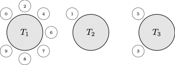
It corresponds to the realised sample, and we certainly wouldn’t want to
break any pedagogical regulations.
Encoding, First Attempt
A natural way to encode the process is to seat each arriving customer at
a new table with the appropriate probability, and then, if it turns out
he is to be sat at an occupied table, to do that with the appropriate
conditional probability (i.e., conditional on the fact that he’s not
going to be seated at a new table).
So let’s imagine encoding a CRP with dispersion parameter ‘a’ and total
number of customers ‘n’. Our first attempt might go something like this:
crp n a = ana coalg (1, <initial restaurant>) where
  coalg (customer, tables)
    | customer >= n = TF.Pure tables
    | otherwise =
        let p = <probability of seating customer at new table>
        in  TF.Free (BernoulliF p (\accept ->
              if   accept
              then (succ customer, <seat at new table>)
              else ???
            ))
We run into a problem when we hit the ‘else’ branch of the conditional.
Here we want to express another random choice – viz., at which occupied
table do we seat the arriving customer. We’d want to do something like
‘TF.Free (UniformF (\u -> …))’ in that ‘else’ branch and then use the
produced uniform value to choose between the occupied tables based on
their conditional probabilities. But that will prove to be impossible,
given the type requirements.
There’s similarly no way to restructure things by producing the
desired uniform value earlier, before the conditional expression. For
appropriate type ‘t’, the coalgebra used for the anamorphism must have
type:
which in our case reduces to:
coalg :: a -> TF.FreeF ModelF a a
You’ll find that there’s simply no way to add another TF.Free
constructor to the mix while satisfying the above type. So it seems that
with an anamorphism (or apomorphism, which encounters the same problem)
we’re limited to denoting a single probabilistic operation on any
recursive call.
Encoding, Correctly
We thus need a recursion scheme that allows us to add multiple levels of
the base functor at a time. The most appropriate scheme appears to me
to be the futumorphism, which I also wrote about in Time Traveling
Recursion Schemes.
(As Patrick Thomson pointed out in his sublime series on
recursion schemes, both anamorphisms and apomorphisms are special cases
of the futumorphism.)
The coalgebra used by a futumorphism has a different type than that used
by an ana- or apomorphism, namely:
coalg :: a -> Base t (Free (Base t) a)
In our case, this is:
coalg :: a -> TF.FreeF ModelF a (Free (TF.FreeF ModelF a) a)
Note that here we’ll be able to use additional ‘TF.Free’ constructors
inside other expressions involving the base functor. In Time Traveling
Recursion Schemes I referred to this as “working with values that
don’t exist yet, while pretending like they do” – but better would
be to say that one is simply defining values to be produced during
(co)recursion, using separate monadic code.
Here’s how we’d encode the CRP using a futumorphism, in pseudocode:
crp n a = futu coalg (1, <initial restaurant>) where
  coalg (customer, tables)
    | customer >= n = TF.Pure tables
    | otherwise =
        let p = <probability of seating customer at new table>
        in  TF.Free (BernoulliF p (\accept ->
              if   accept
              then pure (succ customer, <seat at new table>)
              else do
                res <- liftF (TF.Free (UniformF (\u ->
                         <seat amongst occupied tables using 'u'>
                       )))
                pure (succ customer, res)))
Note that recursive points are expressed under a ‘TF.Free’ constructor
by returning a value (using ‘pure’) in the free monad itself. This
effectively allows us to use more than one embedded language construct
on each recursive call – as many as we want, as a matter of fact. The
familiar ‘liftF’ function lifts each such expression into the free
monad for us.
I mentioned in Time Traveling Recursion Schemes that this sort of
thing can look a little bit nicer if you have the appropriate embedded
language terms floating around. If we define the following:
uniform :: Free (TF.FreeF ModelF a) Double
uniform = liftF (TF.Free (UniformF id))
then we can use it to tidy things up a bit:
crp n a = futu coalg (1, <initial restaurant>) where
  coalg (customer, tables)
    | customer >= n = TF.Pure tables
    | otherwise =
        let p = <probability of seating customer at new table>
        in  TF.Free (BernoulliF p (\accept ->
              if   accept
              then pure (succ customer, <seat at new table>)
              else do
                u <- uniform
                let res = <seat amongst occupied tables using 'u'>
                pure (succ customer, res)))
In any case, the futumorphism gets us to a faithfully-encoded CRP.
It allows us to express multiple probabilistic operations in every
recursive call, which is what’s required here due to our use of
conditional probabilities.
Alternative Encodings
Now. Recall that I mentioned the following:
A natural way to encode the process is to seat each arriving customer
at a new table with the appropriate probability, and then, if it
turns out he is to be sat at an occupied table, to do that with the
appropriate conditional probability (i.e., conditional on the fact
that he’s not going to be seated at a new table).
This is probably the most natural way to encode the process, and indeed,
if we only have Bernoulli and uniform language terms (or beta, Gaussian,
etc. in place of uniform – something that can at least be transformed
to produce a uniform, in any case), this seems to be the best we can do.
But it is not the only way to encode the CRP. If we have a language
term corresponding to a categorical distribution, then we can instead
choose between a new table and any of the occupied tables simultaneously
using the unconditional probabilities for each.
Let’s adjust our ModelF functor, adding a language term corresponding
to a categorical distribution. It will have as its parameter a list of
probabilities, one for each possible outcome under consideration:
data ModelF r =
    BernoulliF Double (Bool -> r)
  | UniformF (Double -> r)
  | CategoricalF [Double] (Int -> r)
  deriving Functor
With this we’ll be able to encode the CRP using a mere anamorphism, as
the following pseudocode describes:
crp n a = ana coalg (1, <initial restaurant>) where
  coalg (customer, tables)
    | customer >= n = TF.Pure tables
    | otherwise =
        let ps = <unconditional categorical probabilities>
        in  TF.Free (CategoricalF ps (\i ->
              if   i == 0
              then (succ customer, <seat at new table>)
              else (succ customer, <seat at occupied table 'i - 1'>)
            ))
Since here we only ever express a single probabilistic term during
recursion, the “standard” pattern we’ve used previously applies here.
But it’s worth noting that we could still employ the “unconditional,
then conditional” approach using a categorical distribution – we’d just
use the conditional probabilities to sample from the occupied tables
directly, rather than doing it in more low-level fashion using the
single uniform draw. Given an appropriate ‘categorical’ term, that would
look more like:
crp n a = futu coalg (1, <initial restaurant>) where
  coalg (customer, tables)
    | customer >= n = TF.Pure tables
    | otherwise =
        let p = <probability of seating customer at new table>
        in  TF.Free (BernoulliF p (\accept ->
              if   accept
              then pure (succ customer, <seat at new table>)
              else do
                let ps = <conditional categorical probabilities>
                i <- categorical ps
                pure (succ customer, <seat at occupied table 'i'>)))
The recursive structure in this case is more complicated, requiring a
futumorphism instead of an anamorphism, but typically the conditional
probabilities are easier to compute.
Fin
So, some takeaways here, if one wants to indulge in this sort of
framework:
If we want to express a stochastic process using multiple probabilistic
operations in any given recursive call, we may need to employ a
scheme that supports richer (co)recursion than a plain anamorphism
or apomorphism. Here that’s captured nicely by a futumorphism, which
naturally captures what we’re looking for.
The same might be true if our functor is sufficiently limited, as
was the case here if we supported only the Bernoulli and uniform
distributions. There we had no option but to express the recursion using
condiitonal probabilistic operations, and so needed the richer recursive
structure that a futumorphism provides.
On the other hand, it may not be the case that one needs the richer
structure provided by a futumorphism, if instead one can express the
coalgebra using only a single layer of the base functor. Adding a
primitive categorical distribution to our embedded language eliminated
the need to use conditional probabilities when describing the recursion,
allowing us to drop back to a “basic” anamorphism.
Here is a gist containing a fleshed-out version of the code
above, if you’d like to play with it. Enjoy!
25 Feb 2020
Long ago, in the distant past, Curtis introduced the idea of kelvin
versioning in an informal blog post about Urbit. Imagining
the idea of an ancient and long-frozen form of Martian computing, he described
this versioning scheme as follows:
Some standards are extensible or versionable, but some are not. ASCII, for
instance, is perma-frozen. So is IPv4 (its relationship to IPv6 is little
more than nominal - if they were really the same protocol, they’d have the
same ethertype). Moreover, many standards render themselves incompatible in
practice through excessive enthusiasm for extensibility. They may not be
perma-frozen, but they probably should be.
The true, Martian way to perma-freeze a system is what I call Kelvin
versioning. In Kelvin versioning, releases count down by integer degrees
Kelvin. At absolute zero, the system can no longer be changed. At 1K, one
more modification is possible. And so on. For instance, Nock is at 9K. It
might change, though it probably won’t. Nouns themselves are at 0K - it is
impossible to imagine changing anything about those three sentences.
Understood in this way, kelvin versioning is very simple. One simply counts
downwards, and at absolute zero (i.e. 0K) no other releases are legal. It is
no more than a versioning scheme designed for abstract components that should
eventually freeze.
Many years later, the Urbit blog described kelvin versioning once more in the
post Towards a Frozen Operating System. This presented a significant
refinement of the original scheme, introducing both recursive and so-called
“telescoping” mechanics to it:
The right way for this trunk to approach absolute zero is to “telescope” its
Kelvin versions. The rules of telescoping are simple:
If tool B sits on platform A, either both A and B must be at absolute zero,
or B must be warmer than A.
Whenever the temperature of A (the platform) declines, the temperature of B
(the tool) must also decline.
B must state the version of A it was developed against. A, when loading B,
must state its own current version, and the warmest version of itself with
which it’s backward-compatible.
Of course, if B itself is a platform on which some higher-level tool C
depends, it must follow the same constraints recursively.
This is more or less a complete characterisation of kelvin versioning, but it’s
still not quite precise enough. If one looks at other versioning schemes that
try to communicate some specific semantic content (the most obvious example
being semver), it’s obvious that they take great pains to be formal and
precise about their mechanics.
Experience has demonstrated to me that such formality is necessary. Even the
excerpt above has proven to be ambiguous or underspecified re: the details of
various situations or corner cases that one might run into. These confusions
can be resolved by a rigorous protocol specification, which, in this case isn’t
very difficult to put together.
Kelvin versioning and its use in Urbit is the subject of the currently-evolving
UP9, recent proposed updates to which have not yet been ratified. The
following is my own personal take on and simple formal specification of kelvin
versioning – I believe it resolves any major ambiguities that the original
descriptions may have introduced.
Kelvin Versioning (Specification)
(The key words “MUST”, “MUST NOT”, “REQUIRED”, “SHALL”, “SHALL NOT”, “SHOULD”,
“SHOULD NOT”, “RECOMMENDED”, “MAY”, and “OPTIONAL” in this document are to be
interpreted as described in RFC 2119.)
For any component A following kelvin versioning,
-
A’s version SHALL be a nonnegative integer.
-
A, at any specific version, MUST NOT be modified after release.
-
At version 0, new versions of A MUST NOT be released.
-
New releases of A MUST be assigned a new version, and this version
MUST be strictly less than the previous one.
-
If A supports another component B that also follows kelvin versioning, then:
- Either both A and B MUST be at version 0, or B’s version MUST be
strictly greater than A’s version.
- If a new version of A is released and that version supports B, then a new
version of B MUST be released.
These rules apply recursively for any kelvin-versioned component C that is
supported by B, and so on.
Examples
Examples are particularly useful here, so let me go through a few.
Let’s take the following four components, sitting in three layers, as a running
example. Here’s our initial state:
So we have A at 10K supporting B at 20K. B in turn supports both C at 21K and
D at 30K.
State 1
Imagine we have some patches lying around for D and want to release a new
version of it. That’s easy to do; we push out a new version of D. In this
case it will have version one less than 30, i.e. 29K:
A       10K
  B     20K
    C   21K
    D   29K  <-- cools from 30K to 29K
Easy peasy. This is the most trivial example.
The only possible point of confusion here is: well, what kind of change
warrants a version decrement? And the answer is: any (released) change
whatsoever. Anything with an associated kelvin version is immutable after
being released at that version, analogous to how things are done in any other
versioning scheme.
State 2
For a second example, imagine that we now have completed a major refactoring
of A and want to release a new version of that.
Since A supports B, releasing a new version of A obligates us to release a new
version of B as well. And since B supports both C and D, we are obligated,
recursively, to release new versions of those to boot.
The total effect of a new A release is thus the following:
A       9K   <-- cools from 10K to 9K
  B     19K  <-- cools from 20K to 19K
    C   20K  <-- cools from 21K to 20K
    D   28K  <-- cools from 29K to 28K
This demonstrates the recursive mechanic of kelvin versioning.
An interesting effect of the above mechanic, as described in Toward a Frozen
Operating System is that anything that depends on (say) A, B, and C only
needs to express its dependency on some version of C. Depending on C at e.g.
20K implicitly specifies a dependency on its supporting component, B, at 19K,
and then A at 9K as well (since any change to A or B must also result in a
change to C).
State 3
Now imagine that someone has contributed a performance enhancement to C, and
we’d like to release a new version of that.
The interesting thing here is that we’re prohibited from releasing a new
version of C. Recall our current state:
A       9K
  B     19K
    C   20K  <-- one degree K warmer than B
    D   28K
Releasing a new version of C would require us to cool it by at least one
kelvin, resulting in the warmest possible version of 19K. But since its
supporting component, B, is already at 19K, this would constitute an illegal
state under kelvin versioning. A supporting component must always be strictly
cooler than anything it supports, or be at absolute zero conjointly with
anything it supports.
This illustrates the so-called telescoping mechanic of kelvin versioning – one
is to imagine one of those handheld telescopes made of segments that flatten
into each other when collapsed.
State 4
But now, say that we’re finally going to release our new API for B. We release
a new version of B, this one at 18K, which obligates us to in turn release new
versions of C and D:
A       9K
  B     18K  <-- cools from 19K to 18K
    C   19K  <-- cools from 20K to 19K
    D   27K  <-- cools from 28K to 27K
In particular, the new version of B gives us the necessary space to release a
new version of C, and, indeed, obligates us to release a new version of it. In
releasing C at 19K, presumably we’d include the performance enhancement that we
were prohibited from releasing in State 3.
State 5
A final example that’s simple, but useful to illustrate explicitly, involves
introducing a new component, or replacing a component entirely.
For example: say that we’ve decided to deprecate C and D and replace them with
a single new component, E, supported by B. This is as easy as it sounds:
A       9K
  B     18K
    E   40K  <-- initial release at 40K
We just swap in E at the desired initial kelvin version. The initial kelvin
can be chosen arbitrarily; the only restriction is that it be warmer than the
the component that supports it (or be at absolute zero conjointly with it).
It’s important to remember that, in this component-resolution of kelvin
versioning, there is no notion of the “total temperature” of the stack. Some
third party could write another component, F, supported by E, with initial
version at 1000K, for example. It doesn’t introduce any extra burden or
responsibility on the maintainers of components A through E.
Collective Kelvin Versioning
So – all that is well and good for what I’ll call the component-level
mechanics of kelvin versioning. But it’s useful to touch on a related
construct, that of collectively versioning a stack of kelvin-versioned
components. This minor innovation on Curtis’s original idea was put together
by myself and my colleague Philip Monk.
If you have a collection of kelvin-versioned things, e.g. the things in our
initial state from the prior examples:
then you may want to release all these things, together, as some abstract
thing. Notably, this happens in the case of the Urbit kernel, where the stack
consists of a functional VM, an unapologetically amathematical purely
functional programming language, special-purpose kernel modules, etc.
It’s useful to be able to describe the whole kernel with a single version
number.
To do this in a consistent way, you can select one component in your stack to
serve as a primary index of sorts, and then capture everything it supports via
a patch-like, monotonically decreasing “fractional temperature” suffix.
This is best illustrated via example. If we choose B as our primary index in
the initial state above, for example, we could version the stack collectively
as 20.9K. B provides the 20K, and everything it supports is just lumped into
the “patch version” 9.
If we then consider the example given in State 1, i.e.:
in which D has cooled by a degree kelvin, then we can version this stack
collectively as 20.8K. If we were to then release a new version of C at 20K,
then we could release the stack collectively as 20.7K. And so on.
There is no strictly prescribed schedule as to how to decrease the fractional
temperature, but the following schedule is recommended:
.9, .8, .7, .., .1, .01, .001, .0001, ..
Similarly, the fractional temperature should reset to .9 whenever the primary
index cools. If we consider the State 2, for example, where a new release of A
led to every other component in the stack cooling, we had this:
Note that B has cooled by a kelvin, so we would version this stack collectively
as 19.9K. The primary index has decreased by a kelvin, and the fractional
temperature has been reset to .9.
While I think examples illustrate this collective scheme most clearly, after my
schpeel about the pitfalls of ambiguity it would be remiss of me not to include
a more formal spec:
Collective Kelvin Versioning (Specification)
(The key words “MUST”, “MUST NOT”, “REQUIRED”, “SHALL”, “SHALL NOT”, “SHOULD”,
“SHOULD NOT”, “RECOMMENDED”, “MAY”, and “OPTIONAL” in this document are to be
interpreted as described in RFC 2119.)
For a collection of kelvin-versioned components K:
-
K’s version SHALL be characterised by a primary index, chosen from a
component in K, and and a real number in the interval [0, 1) (the
“fractional temperature”), determined by all components that the primary
index component supports.
The fractional temperature MAY be 0 only if the primary index’s version
is 0.
-
K, at any particular version, MUST NOT be modified after release.
-
At primary index version 0 and fractional temperature 0, new versions of K
MUST NOT be released.
-
New releases of K MUST be assigned a new version, and this version
MUST be strictly less than the previous one.
-
When a new release of K includes new versions of any component supported by
the primary index, but not a new version of the primary index proper, its
fractional temperature MUST be less than the previous version.
Given constant primary index versions, fractional temperatures corresponding
to new releases SHOULD decrease according to the following schedule:
.9, .8, .7, .., .1, .01, .001, .0001, ..
-
When a new release of K includes a new version of the primary index, the
fractional temperature of SHOULD be reset to 9.
-
New versions of K MAY be indexed by components other than the primary
index (i.e., K may be “reindexed” at any point). However, the new chosen
component MUST either be colder than the primary index it replaces, or
be at version 0 conjointly with the primary index it replaces.
Etc.
In my experience, the major concern in adopting a kelvin versioning scheme is
that one will accidentally initialise everything with a set of temperatures
(i.e. versions) that are too cold (i.e. too close to 0), and thus burn through
too many version numbers too quickly on the path to freezing. To alleviate
this, it helps to remember that one has an infinite number of release
candidates available for every component at every temperature.
The convention around release candidates is just to prepend a suffix to the
next release version along the lines of .rc1, .rc2, etc. One should feel
comfortable using these liberally, iterating through release candidates as
necessary before finally committing to a new version at a properly cooler
temperature.
The applications that might want to adopt kelvin versioning are probably pretty
limited, and may indeed even be restricted to the Urbit kernel itself (Urbit
has been described by some as “that operating system with kernel that
eventually reaches absolute zero under kelvin versioning”). Nonetheless: I
believe this scheme to certainly be more than a mere marketing gimmick or what
have you, and, at minimum, it makes for an interesting change of pace from
semver.