Transforming to CPS

I recently picked up Appel’s classic Compiling with Continuations and have been refreshing my continuation-fu more generally.

Continuation-passing style (CPS) itself is nothing uncommon to the functional programmer; it simply involves writing in a manner such that functions never return, instead passing control over to something else (a continuation) to finish the job. The simplest example is just the identity function, which in CPS looks like this:

id :: a -> (a -> b) -> b
id x k = k x

The first argument is the conventional identity function argument – the second is the continuation. I wrote a little about continuations in the context of the Giry monad, which is a somewhat unfamiliar setting, but one that follows the same principles as anything else.

In this post I just want to summarise a few useful CPS transforms and related techniques in one place.

Manual CPS Transformation

Consider a binary tree type. We’ll keep things simple here:

data Tree a =
    Leaf a
  | Branch a (Tree a) (Tree a)

Calculating the depth of a tree is done very easily:

depth :: Tree a -> Int
depth = loop where
  loop tree = case tree of
    Leaf _       -> 1
    Branch _ l r ->
      let dl = loop l
          dr = loop r
      in  succ (max dl dr)

Note however that this is not a tail-recursive function – that is, it does not end with a call to itself (instead it ends with a call to something like ‘succ . uncurry max’). This isn’t necessarily a big deal – the function is easy to read and write and everything, and certainly has fine performance characteristics in Haskell – but it is less easy to deal with for, say, an optimising compiler that may want to handle evaluation in this or that alternative way (primarily related to memory management).

One can construct a tail-recursive (depth-first) version of ‘depth’ via a manual CPS transformation. The looping function is simply augmented to take an additional continuation argument, like so:

depth :: Tree a -> Int
depth tree = loop tree id where
  loop cons k = case cons of
    Leaf _       -> k 1
    Branch _ l r ->
      loop l $ \dl ->
        loop r $ \dr ->
          k (succ (max dl dr))

Notice now that the ‘loop’ function terminates with a call to itself (or just passes control to a supplied continuation), and is thus tail-recursive.

Due to the presence of the continuation argument, ‘loop’ is a higher-order function. This is fine and dandy in Haskell, but there is a neat technique called defunctionalisation that allows us to avoid the jump to higher-order and makes sure things stay KILO (“keep it lower order”), which can be simpler to deal with more generally.

The idea is just to reify the continuations as abstract syntax, and then evaluate them as one would any embedded language. Note the continuation \dl -> .., for example – the free parameters ‘r’ and ‘k’ occuring in the function body correspond to a tree (the right subtree) and another continuation, respectively. And in \dr -> .. one has the free parameters ‘dl’ and ‘k’ – now the depth of the left subtree, and the other continuation again. We also have ‘id’ used on the initial call to ‘loop’. These can all be reified via the following data type:

data DCont a =
    DContL (Tree a) (DCont a)
  | DContR Int (DCont a)
  | DContId

Note that this is a very simple recursive type – it has a simple list-like pattern of recursion, in which each ‘level’ of a value is either a constructor, carrying both a field of some type and a recursive point, or is the ‘DContId’ constructor, which simply terminates the recursion. The reified continuations are, on a suitable level of abstraction, more or less the sequential operations to be performed in the computation. In other words: by reifying the continuations, we also reify the stack of the computation.

Now ‘depth’ can be rewritten such that its looping function is not higher-order; the cost is that another function is needed, one that lets us evaluate items (again, reified continuations) on the stack:

depth :: Tree a -> Int
depth tree = loop tree DContId where
  loop cons k = case cons of
    Leaf _       -> eval k 1
    Branch _ l r -> loop l (DContL r k)

  eval cons d = case cons of
    DContL r k  -> loop r (DContR d k)
    DContR dl k -> eval k (succ (max dl d))
    DContId     -> d

The resulting function is mutually tail-recursive in terms of both ‘loop’ and ‘eval’, neither of which are higher-order.

One can do a little better in this particular case and reify the stack using an actual Haskell list, which simplifies evaluation somewhat – it just requires that the list elements have a type along the lines of ‘(Tree a, Int)’ rather than something like ‘Either (Tree a) Int’, which is effectively what we get from ‘DCont a’. You can see an example of this in this StackOverflow answer by Chris Taylor.

Mechanical CPS Transformation

“Mechanical CPS transformation” might be translated as simply “compiling with continuations.” Matt Might has quite a few posts on this topic; in particular he has one very nice post on mechanical CPS conversion that summarises various transformations described in Appel, etc.

Matt describes three transformations that I think illustrate the general mechanical CPS business very well (he describes more, but they are more specialised). The first is a “naive” transformation, which is simple, but produces a lot of noisy “administrative redexes” that must be cleaned up in another pass. The second is a higher-order transformation, which makes use of the host language’s facilities for function definition and application – it produces simpler code, but some unnecessary noise still leaks through. The last is a “hybrid” transformation, which makes use of both the naive and higher-order transformations, depending on which is more appropriate.

Let’s take a look at these in Haskell. First let’s get some imports out of the way:

{-# LANGUAGE OverloadedStrings #-}

import Data.Monoid
import Data.Text (Text)
import qualified Data.Text as T
import Data.Unique
import qualified Text.PrettyPrint.Leijen.Text as PP

I’ll also make use of a simple, Racket-like ‘gensym’ function:

gensym :: IO Text
gensym = fmap render newUnique where
  render u =
    let hu = hashUnique u
    in  T.pack ("$v" <> show hu)

We’ll use a bare-bones lambda calculus as our input language. Many examples – Appel’s especially – use significantly more complex languages when illustrating CPS transforms, but I think this distracts from the meat of the topic. Lambda does just fine:

data Expr =
    Lam Text Expr
  | Var Text
  | App Expr Expr

I want to render expressions in my input and output languages in a Lisp-like manner. This is very easy to do using a good pretty-printing library; here I’m using the excellent wl-pprint-text, and will omit the ‘Pretty’ instances in the body of my post. But I’ll link to a gist including them at the bottom.

When performing a mechanical CPS transform, one targets both “atomic” expressions – i.e., variables and lambda abstractions – and “complex” expressions, i.e. function application. The target language is thus a combination of the ‘AExpr’ and ‘CExpr’ types:

data AExpr =
    AVar Text
  | ALam [Text] CExpr

data CExpr =
    CApp AExpr [AExpr]

All the mechanical CPS transformations use variants on two functions going by the cryptic names m and t. m is responsible for converting atomic expressions in the input languages (i.e., variables and lambda abstractions) into atomic expressions in the target language (an atomic CPS expression). t is the actual CPS transformation; it converts an expression in the input language into CPS, invoking a specified continuation (already in the target language) on the result.

Let’s look at the naive transform. Here are m and t, prefixed by ‘n’ to indicate that they are naive. First, m:

nm :: Expr -> IO AExpr
nm expr = case expr of
  Lam var cexpr0 -> do
    k      <- gensym
    cexpr1 <- nt cexpr0 (AVar k)
    return (ALam [var, k] cexpr1)

  Var var -> return (AVar var)

  App {} -> error "non-atomic expression"

(N.b. you almost never want to use ‘error’ in a production implementation of anything. It’s trivial to wrap e.g. ‘MaybeT’ around the appropriate functions to handle the bogus pattern match on ‘App’ totally, but I just want to keep the types super simple here.)

The only noteworthy thing that m does here is in the case of a lambda abstraction: a new abstract continuation is generated, and the body of the abstraction is converted to CPS via t, such that the freshly-generated continuation is called on the result. Remember, m is really just mapping atomic expressions in the input language to atomic expressions in the target language.

Here’s t for the naive transform. Remember, t is responsible for converting expressions to continuation-passing style:

nt :: Expr -> AExpr -> IO CExpr
nt expr cont = case expr of
  Lam {} -> do
    aexpr <- m expr
    return (CApp cont [aexpr])

  Var _ -> do
    aexpr <- m expr
    return (CApp cont [aexpr])

  App f e -> do
    fs <- gensym
    es <- gensym

    let aexpr0 = ALam [es] (CApp (AVar fs) [AVar es, cont])

    cexpr <- nt e aexpr0

    let aexpr1 = ALam [fs] cexpr

    nt f aexpr1

For both kinds of atomic expressions (lambda and variable), the expression is converted to the target language via m, and then the supplied continuation is applied to it. Very simple.

In the case of function application (a “complex”, or non-atomic expression), both the function to be applied, and the argument it is to be applied to, must be converted to CPS. This is done by generating two fresh continuations, transforming the argument, and then transforming the function. The control flow here is always handled by stitching continuations together; notice when transforming the function ‘f’ that the continuation to be applied has already handled its argument.

Next, the higher-order transform. Here are m and t:

hom :: Expr -> IO AExpr
hom expr = case expr of
  Lam var e -> do
    k  <- gensym
    ce <- hot e (\rv -> return (CApp (AVar k) [rv]))
    return (ALam [var, k] ce)

  Var n  -> return (AVar n)

  App {} -> error "non-atomic expression"

hot :: Expr -> (AExpr -> IO CExpr) -> IO CExpr
hot expr k = case expr of
  Lam {} -> do
    aexpr <- m expr
    k aexpr

  Var {} -> do
    aexpr <- m expr
    k aexpr

  App f e -> do
    rv      <- gensym
    xformed <- k (AVar rv)

    let cont = ALam [rv] xformed

        cexpr fs = hot e (\es -> return (CApp fs [es, cont]))

    hot f cexpr

Both of these have the same form as they do in the naive transform – the difference here is simply that the continuation to be applied to a transformed expression is expressed in the host language – i.e., here, Haskell. Thus the transform is “higher-order,” in exactly the same sense that higher-order abstract syntax is higher-order.

The final transformation I’ll illustrate here, the hybrid transform, applies the naive transformation to lambda and variable expressions, and applies the higher-order transformation to function applications. Here t is split up into tc and tk to handle these cases accordingly:

m :: Expr -> IO AExpr
m expr = case expr of
  Lam var cexpr -> do
    k       <- gensym
    xformed <- tc cexpr (AVar k)
    return (ALam [var, k] xformed)

  Var n  -> return (AVar n)

  App {} -> error "non-atomic expression"

tc :: Expr -> AExpr -> IO CExpr
tc expr c = case expr of
  Lam {} -> do
    aexpr <- m expr
    return (CApp c [aexpr])

  Var _ -> do
    aexpr <- m expr
    return (CApp c [aexpr])

  App f e -> do
    let cexpr fs = tk e (\es -> return (CApp fs [es, c]))
    tk f cexpr

tk :: Expr -> (AExpr -> IO CExpr) -> IO CExpr
tk expr k = case expr of
  Lam {} -> do
    aexpr <- m expr
    k aexpr

  Var {} -> do
    aexpr <- m expr
    k aexpr

  App f e -> do
    rv <- gensym
    xformed <- k (AVar rv)

    let cont     = ALam [rv] xformed
        cexpr fs = tk e (\es -> return (CApp fs [es, cont]))

    tk f cexpr

Matt illustrates these transformations on a simple expression: (g a). We can do the same:

test :: Expr
test = App (Var "g") (Var "a")

First, the naive transform. Note all the noisy administrative redexes that come along with it:

> cexpr <- nt test (AVar "halt")
> PP.pretty cexpr
((λ ($v1).
  ((λ ($v2).
    ($v1 $v2 halt)) a)) g)

The higher-order transform does better, containing only one such redex (an eta-expansion). Note that since the supplied continuation must be expressed in terms of a Haskell function, we need to write it in a more HOAS-y style:

> cexpr <- hot test (\ans -> return (CApp (AVar "halt") [ans]))
> PP.pretty cexpr
(g a (λ ($v3).
  (halt $v3)))

Finally the hybrid transform, which, here, is literally perfect. We don’t even need to deal with the minor annoyance of the HOAS-style continuation when calling it:

> cexpr <- tc test (AVar "halt")
> PP.pretty cexpr
(g a halt)

Matt goes on to describe a “partioned CPS transform” that can be used to recover a stack, in (seemingly) much the same manner that the defunctionalised manual CPS transform worked in the previous section. Very neat, but something I’ll have to look at in another post.

Fin

CPS is pretty gnarly. My experience in compiling with continuations is not substantial, but I dig learning it. Appel’s book, in particular, is meaty – expect more posts on the subject here eventually, probably.

‘Til next time! I’ve dumped the code from the latter section into a gist.

Embedded DSLs for Bayesian Modelling and Inference: a Retrospective

Why does my blog often feature its typical motley mix of probability, functional programming, and computer science anyway?

From 2011 through 2017 I slogged through a Ph.D. in statistics, working on it full time in 2012, and part-time in every other year. It was an interesting experience. Although everything worked out for me in the end – I managed to do a lot of good and interesting work in industry while still picking up a Ph.D. on the side – it’s not something I’d necessarily recommend to others. The smart strategy is surely to choose one thing and give it one’s maximum effort; by splitting my time between work and academia, both obviously suffered to some degree.

That said, at the end of the day I was pretty happy with the results on both fronts. On the academic side of things, the main product was a dissertation, Embedded Domain-Specific Languages for Bayesian Modelling and Inference, supporting my thesis: that novel and useful DSLs for solving problems in Bayesian statistics can be embedded in statically-typed, purely functional programming languages.

It helps to remember that in this day and age, one can still typically graduate by, uh, “merely” submitting and defending a dissertation. Publishing in academic venues certainly helps focus one’s work, and is obviously necessary for a career in academia (or, increasingly, industrial research). But it’s optional when it comes to getting your degree, so if it doesn’t help you achieve your goals, you may want to reconsider it, as I did.

The problem with the dissertation-first approach, of course, is that nobody reads your work. To some extent I think I’ve mitigated that; most of the content in my dissertation is merely a fleshed-out version of various ideas I’ve written about on this blog. Here I’ll continue that tradition and write a brief, informal summary of my dissertation and Ph.D. more broadly – what I did, how I approached it, and what my thoughts are on everything after the fact.

The Idea

Following the advice of Olin Shivers (by way of Matt Might), I oriented my work around a concrete thesis, which wound up more or less being that embedding DSLs in a Haskell-like language can be a useful technique for solving statistical problems. This thesis wasn’t born into the world fully-formed, of course – it began as quite a vague (or misguided) thing, but matured naturally over time. Using the tools of programming languages and compilers to do statistics and machine learning is the motivation behind probabilistic programming in general; what I was interested in was exploring the problem in the setting of languages embedded in a purely functional host. Haskell was the obvious choice of host for all of my implementations.

It may sound obvious that putting together a thesis is a good strategy for a Ph.D. But here I’m talking about a thesis in the original (Greek) sense of a proposition, i.e. a falsifiable idea or claim (in contrast to a dissertation, from the Latin disserere, i.e. to examine or to discuss). Having a central idea to orient your work around can be immensely useful in terms of focus. When you read a dissertation with a clear thesis, it’s easy to know what the writer is generally on about – without one it can (increasingly) be tricky.

My thesis is pretty easy to defend in the abstract. A DSL really exposes the structure of one’s problem while also constraining it appropriately, and embedding one in a host language means that one doesn’t have to implement an entire compiler toolchain to support it. I reckoned that simply pointing the artillery of “language engineering” at the statistical domain would lead to some interesting insight on structure, and maybe even produce some useful tools. And it did!

The Contributions

Of course, one needs to do a little more defending than that to satisfy his or her examination committee. Doctoral research is supposed to be substantial and novel. In my experience, reviewers are concerned with your answers to the following questions:

• What, specifically, are your claims?
• Are they novel contributions to your field?
• Have you backed them up sufficiently?

At the end of the day, I claimed the following advances from my work.

• Novel probabilistic interpretations of the Giry monad’s algebraic structure. The Giry monad (Lawvere, 1962; Giry, 1981) is the “canonical” probability monad, in a meaningful sense, and I demonstrated that one can characterise the measure-theoretic notion of image measure by its functorial structure, as well as the notion of product measure by its monoidal structure. Having the former around makes it easy to transform the support of a probability distribution while leaving its density structure invariant, and the latter lets one encode probabilistic independence, enabling things like measure convolution and the like. What’s more, the analogous semantics carry over to other probability monads – for example the well-known sampling monad, or more abstract variants.

• A novel characterisation of the Giry monad as a restricted continuation monad. Ramsey & Pfeffer (2002) discussed an “expectation monad,” and I had independently come up with my own “measure monad” based on continuations. But I showed both reduce to a restricted form of the continuation monad of Wadler (1994) – and that indeed, when the return type of Wadler’s continuation monad is restricted to the reals, it is the Giry monad.

  To be precise it’s actually somewhat more general – it permits integration with respect to any measure, not only a probability measure – but that definition strictly subsumes the Giry monad. I also showed that product measure, via the applicative instance, yields measure convolution and associated operations.

• A novel technique for embedding a statically-typed probabilistic programming language in a purely functional language. The general idea itself is well-known to those who have worked with DSLs in Haskell: one constructs a base functor and wraps it in the free monad. But the reason that technique is appropriate in the probabilistic programming domain is that probabilistic models are fundamentally monadic constructs – merely recall the existence of the Giry monad for proof!

  To construct the requisite base functor, one maps some core set of concrete probability distributions denoted by the Giry monad to a collection of abstract probability distributions represented only by unique names. These constitute the branches of one’s base functor, which is then wrapped in the familiar ‘Free’ machinery that gives one access to the functorial, applicative, and monadic structure that I talked about above. This abstract representation of a probabilistic model allows one to implement other probability monads, such as the well-known sampling monad (Ramsey & Pfeffer, 2002; Park et al., 2008) or the Giry monad, by way of interpreters.

  (N.b. Ścibior et al. (2015) did some very similar work to this, although the monad they used was arguably more operational in its flavour.)

• A novel characterisation of execution traces as cofree comonads. The idea of an “execution trace” is that one runs a probabilistic program (typically generating a sample) and then records how it executed – what randomness was used, the execution path of the program, etc. To do Bayesian inference, one then runs a Markov chain over the space of possible execution traces, calculating statistics about the resulting distribution in trace space (Wingate et al., 2011).

  Remarkably, a cofree comonad over the same abstract probabilistic base functor described above allows us to represent an execution trace at the embedded language level itself. In practical terms, that means one can denote a probabilistic model, and then run a Markov chain over the space of possible ways it could have executed, without leaving GHCi. You can alternatively examine and perturb the way the program executes, stepping through it piece by piece, as I believe was originally a feature in Venture (Mansinghka et al., 2014).

  (N.b. this really blew my mind when I first started toying with it, converting programs into execution traces and then manipulating them as first-class values, defining other probabilistic programs over spaces of execution traces, etc. Meta.)

• A novel technique for statically encoding conditional independence of terms in this kind of embedded probabilistic programming language. If you recall that I previously demonstrated the monoidal (i.e. applicative) structure of the Giry monad encodes the notion of product measure, it will not be too surprising to hear that I used the free applicative functor (Capriotti & Kaposi, 2014) (again, over the same kind of abstract probabilistic base functor) to reify applicative expressions such that they can be identified statically.

• A novel shallowly-embedded language for building custom transition operators for use in Markov chain Monte Carlo. MCMC is the de-facto standard way to perform inference on Bayesian models (although it is not limited to Bayesian models in particular). By wrapping a simple state monad transformer around a probability monad, one can denote Markov transition operators, combine them, and transform them in a few ways that are useful for doing MCMC.

  The framework here was inspired by the old parallel “strategies” idea of Trinder et al. (1998). The idea is that you want to “evaluate” a posterior via MCMC, and want to choose a strategy by which to do so – e.g. Metropolis (Metropolis, 1953), slice sampling (Neal, 2003), Hamiltonian (Neal, 2011), etc. Since Markov transition operators are closed under composition and convex combinations, it is easy to write a little shallowly-embedded combinator language for working with them – effectively building evaluation strategies in a manner familiar to those who’ve worked with Haskell’s parallel library.

  (N.b. although this was the most trivial part of my research, theoretical or implementation-wise, it remains the most useful for day-to-day practical work.)

The Execution

One needs to stitch his or her contributions together in some kind of over-arching narrative that supports the underlying thesis. Mine went something like this:

The Giry monad is appropriate for denoting probabilistic semantics in languages with purely-functional hosts. Its functorial, applicative, and monadic structure denote probability distributions, independence, and marginalisation, respectively, and these are necessary and sufficient for encoding probabilistic models. An embedded language based on the Giry monad is type-safe and composable.

Probabilistic models in an embedded language, semantically denoted in terms of the Giry monad, can be made abstract and interpretation-independent by defining them in terms of a probabilistic base functor and a free monad instead. They can be forward-interpreted using standard free monad recursion schemes in order to compute probabilities (via a measure intepretation) or samples (via a sampling interpretation); the latter interpretation is useful for performing limited forms of Bayesian inference, in particular. These free-encoded models can also be transformed into cofree-encoded models, under which they represent execution traces that can be perturbed arbitrarily by standard comonadic machinery. This representation is amenable to more elaborate forms of Bayesian inference. To accurately denote conditional independence in the embedded language, the free applicative functor can also be used.

One can easily construct a shallowly-embedded language for building custom Markov transitions. Markov chains that use these compound transitions can outperform those that use only “primitive” transitions in certain settings. The shallowly embedded language guarantees that transitions can only be composed in well-defined, type-safe ways that preserve the properties desirable for MCMC. What’s more, one can implement “transition transformers” for implementing still more complex inference techniques, e.g. annealing or tempering, over existing transitions.

Thus: novel and useful domain-specific languages for solving problems in Bayesian statistics can be embedded in statically-typed, purely-functional programming languages.

I used the twenty-minute talk period of my defence to go through this narrative and point out my claims, after which I was grilled on them for an hour or two. The defence was probably the funnest part of my whole Ph.D.

The Product

In the end, I mainly produced a dissertation, a few blog posts, and some code. By my count, the following repos came out of the work:

• deanie: An embedded probabilistic programming language.
  http://github.com/jtobin/deanie

• declarative: DIY Markov Chains.
  http://github.com/jtobin/declarative

• flat-mcmc: Painless general-purpose sampling.
  http://github.com/jtobin/flat-mcmc

• hasty-hamiltonian: Speedy traversal through parameter space.
  http://github.com/jtobin/hasty-hamiltonian

• hnuts: Automatic gradient-based sampling.
  http://github.com/jtobin/hnuts

• lazy-langevin: Gradient-based diffusion.
  http://github.com/jtobin/lazy-langevin

• mcmc-types: Common types for implementing MCMC algorithms.
  https://github.com/jtobin/mcmc-types

• measurable: A shallowly-embedded DSL for basic measure wrangling.
  http://github.com/jtobin/measurable

• mighty-metropolis: The Metropolis sampling algorithm.
  http://github.com/jtobin/mighty-metropolis

• mwc-probability: Sampling function-based probability distributions.
  http://github.com/jtobin/mwc-probability

• sampling: Tools for sampling from collections.
  https://github.com/jtobin/sampling

• speedy-slice: Speedy slice sampling.
  http://github.com/jtobin/speedy-slice

If any of this stuff is or was useful to you, that’s great! I still use the declarative libraries, flat-mcmc, mwc-probability, and sampling pretty regularly. They’re fast and convenient for practical work.

Some of the other stuff, e.g. measurable, is useful for building intuition, but not so much in practice, and deanie, for example, is a work-in-progress that will probably not see much more progress (from me, at least). Continuing from where I left off might be a good idea for someone who wants to explore problems in this kind of setting in the future.

General Thoughts

When I first read about probabilistic (functional) programming in Dan Roy’s 2011 dissertation I was absolutely blown away by the idea. It seemed that, since there was such an obvious connection between the structure of Bayesian models and programming languages (via the underlying semantic graph structure, something that has been exploited to some degree as far back as BUGS), it was only a matter of time until someone was able to really create a tool that would revolutionize the practice of Bayesian statistics.

Now I’m much more skeptical. It’s true that probabilistic programming tends to expose some beautiful structure in statistical models, and that a probabilistic programming language that was easy to use and “just worked” for inference would be a very useful tool. But putting something expressive and usable together that also “just works” for that inference step is very, very difficult. Very difficult indeed.

Almost every probabilistic programming framework of the past ten years, from Church down to my own stuff, has more or less wound up as “thesisware,” or remains the exclusive publication-generating mechanism of a single research group. The exceptions are almost unexceptional in of themselves: JAGS and Stan are probably the most-used such frameworks, certainly in statistics (I will mention the very honourable PyMC here as well), but they innovate little, if at all, over the original BUGS in terms of expressiveness. Similarly it’s very questionable whether the fancy MCMC algo du jour is really any better than some combination of Metropolis-Hastings (even plain Metropolis), Gibbs (or its approximate variant, slice sampling), or nested sampling in anything outside of favourably-engineered examples (I will note that Hamiltonian Monte Carlo could probably be counted in there too, but it can still be quite a pain to use, its variants are probably overrated, and it is comparatively expensive).

Don’t get me wrong. I am a militant Bayesian. Bayesian statistics, i.e., as far as I’m concerned, probability theory, describes the world accurately. And there’s nothing wrong with thesisware, either. Research is research, and this is a very thorny problem area. I hope to see more abandoned, innovative software that moves the ball up the field, or kicks it into another stadium entirely. Not less. The more ingenious implementations and sampling schemes out there, the better.

But more broadly, I often find myself in the camp of Leo Breiman, who in 2001 characterised the two predominant cultures in statistics as those of data modelling and algorithmic modelling respectively, the latter now known as machine learning, of course. The crux of the data modelling argument, which is of course predominant in probabilistic programming research and Bayesian statistics more generally, is that a practitioner, by means of his or her ingenuity, is able to suss out the essence of a problem and distill it into a useful equation or program. Certainly there is something to this: science is a matter of creating hypotheses, testing them against the world, and iterating on that, and the “data modelling” procedure is absolutely scientific in principle. Moreover, with a hat tip to Max Dama, one often wants to impose a lot of structure on a problem, especially if the problem is in a domain where there is a tremendous amount of noise. There are many areas where this approach is just the thing one is looking for.

That said, it seems to me that a lot of the data modelling-flavoured side of probabilistic programming, Bayesian nonparametrics, etc., is to some degree geared more towards being, uh, “research paper friendly” than anything else. These are extremely seductive areas for curious folks who like to play at the intersection of math, statistics, and computer science (raises hand), and one can easily spend a lifetime chasing this or that exquisite theoretical construct into any number of rabbit holes. But at the end of the day, the data modelling culture, per Breiman:

.. has at its heart the belief that a statistician, by imagination and by looking at the data, can invent a reasonably good parametric class of models for a complex mechanism devised by nature.

Certainly the traditional statistics that Breiman wrote about in 2001 was very different from probabilistic programming and similar fields in 2018. But I think there is the same element of hubris in them, and to some extent, a similar dissociation from reality. I have cultivated some of the applied bent of a Breiman, or a Dama, or a Locklin, so perhaps this should not be too surprising.

I feel that the 2012-ish resurgence of neural networks jolted the machine learning community out of a large-scale descent into some rather dubious Bayesian nonparametrics research, which, much as I enjoy that subject area, seemed more geared towards generating fun machine learning summer school lectures and NIPS papers than actually getting much practical work done. I can’t help but feel that probabilistic programming may share a few of those same characteristics. When all is said and done, answering the question is this stuff useful? often feels like a stretch.

So: onward & upward and all that, but my enthusiasm has been tempered somewhat, is all.

Fini

Administrative headaches and the existential questions associated with grad school aside, I had a great time working in this area for a few years, if in my own aloof and eccentric way.

If you ever interacted with this area of my work, I hope you got some utility out of it: research ideas, use of my code, or just some blog post that you thought was interesting during a slow day at the office. If you’re working in the area, or are considering it, I wish you success, whether your goal is to build practical tools, or to publish sexy papers. :-)

Fubini and Applicatives

Take an iterated integral, e.g. \(\int_X \int_Y f(x, y) dy dx\). Fubini’s Theorem describes the conditions under which the order of integration can be swapped on this kind of thing while leaving its value invariant. If Fubini’s conditions are met, you can convert your integral into \(\int_Y \int_X f(x, y) dx dy\) and be guaranteed to obtain the same result you would have gotten by going the other way.

What are these conditions? Just that you can glue your individual measures together as a product measure, and that \(f\) is integrable with respect to it. I.e.,

Say you have a Giry monad implementation kicking around and you want to see how Fubini’s Theorem works in terms of applicative functors, monads, continuations, and all that. It’s pretty easy. You could start with my old measurable library that sits on GitHub and attracts curious stars from time to time and cook up the following example:

import Control.Applicative ((<$>), (<*>))
import Measurable

dx :: Measure Int
dx = bernoulli 0.5

dy :: Measure Double
dy = beta 1 1

dprod :: Measure (Int, Double)
dprod = (,) <$> dx <*> dy

Note that ‘dprod’ is clearly a product measure (I’ve constructed it using the Applicative instance for the Giry monad, so it must be a product measure) and take a simple, obviously integrable function:

add :: (Int, Double) -> Double
add (m, x) = fromIntegral m + x

Since ‘dprod’ is a product measure, Fubini’s Theorem guarantees that the following are equivalent:

i0 :: Double
i0 = integrate add dprod

i1 :: Double
i1 = integrate (\x -> integrate (curry add x) dy) dx

i2 :: Double
i2 = integrate (\y -> integrate (\x -> curry add x y) dx) dy

And indeed they are – you can verify them yourself if you don’t believe me (or our boy Fubini).

For an example of a where interchanging the order of integration would be impossible, we can construct some other measure:

dpair :: Measure (Int, Double)
dpair = do
  x <- dx
  y <- fmap (* fromIntegral x) dy
  return (x, y)

It can be integrated as follows:

i3 :: Double
i3 = integrate (\x -> integrate (curry add x) (fmap (* fromIntegral x) dy)) dx

But notice how ‘dpair’ is constructed: it is strictly monadic, not applicative, so the order of the expressions matters. Since ‘dpair’ can’t be expressed as a product measure (i.e. by an applicative expression), Fubini says that swapping the order of integration is a no-no.

Note that if you were to just look at the types of ‘dprod’ and ‘dpair’ – both ‘Measure (Int, Double)’ – you wouldn’t be able to tell immediately that one represents a product measure while the other one does not. If being able to tell these things apart statically is important to you (say, you want to statically apply order-of-integration optimisations to integral expressions or what have you), you need look no further than the free applicative functor to help you out.

Fun fact: there is a well-known variant of Fubini’s Theorem, called Tonelli’s Theorem, that was developed by another Italian guy at around the same time. I’m not sure how early-20th century Italy became so strong in order-of-integration research, exactly.

Byzantine Generals and Nakamoto Consensus

You can recognize truth by its beauty and simplicity.

– Richard Feynman (attributed)

In one of his early emails on the Cryptography mailing list, Satoshi claimed that the proof-of-work chain is a solution to the Byzantine Generals Problem (BGP). He describes this via an example where a bunch of generals – Byzantine ones, of course – collude to break a king’s wifi.

It’s interesting to look at this a little closer in the language of the originally-stated BGP itself. One doesn’t need to be too formal to glean useful intuition here.

What, more precisely, did Satoshi claim?

The Decentralized Timestamp Server

Satoshi’s problem is that of a decentralized timestamp server (DTS). Namely, he posits that any number of nodes, following some protocol, can together act as a timestamping server – producing some consistent ordering on what we’ll consider to be abstract ‘blocks’.

The decentralized timestamp server reduces to an instance of the Byzantine Generals Problem as follows. There are a bunch of nodes, who could each be honest or dishonest. All honest nodes want to agree on some ordering – a history – of blocks, and a small number of dishonest nodes should not easily be able to compromise that history – say, by convincing the honest nodes to adopt some alternate one of their choosing.

(N.b. it’s unimportant here to be concerned about the contents of blocks. Since the decentralized timestamp server problem is only concerned about block orderings, we don’t need to consider the case of invalid transactions within blocks or what have you, and can safely assume that any history must be internally consistent. We only need to assume that child blocks depend utterly on their parents, so that rewriting a history by altering some parent block also necessitates rewriting its children, and that honest nodes are constantly trying to append blocks.)

As demonstrated in the introduction to the original paper, the Byzantine Generals Problem can be reduced to the problem of how any given node communicates its information to others. In our context, it reduces to the following:

Byzantine Generals Problem (DTS)

A node must broadcast a history of blocks to its peers, such that:

• (IC1) All honest peers agree on the history.
• (IC2) If the node is honest, then all honest peers agree with the history it broadcasts.

To produce consensus, every node will communicate its history to others by using a solution to the Byzantine Generals Problem.

Longest Proof-of-Work Chain

Satoshi’s proposed solution to the BGP has since come to be known as ‘Nakamoto Consensus’. It is the following protocol:

Nakamoto Consensus

• Always use the longest history.
• Appending a block to any history requires a proof that a certain amount of work – proportional in expectation to the total ‘capability’ of the network – has been completed.

To examine how it works, consider an abstract network and communication medium. We can assume that messages are communicated instantly (it suffices that communication is dwarfed in time by actually producing a proof of work) and that the network is static and fixed, so that only active or ‘live’ nodes actually contribute to consensus.

The crux of Nakamoto consensus is that nodes must always use the longest available history – the one that provably has the largest amount of work invested in it – and appending to any history requires a nontrivial amount of work in of itself. Consider a set of nodes, each having some (not necessarily shared) history. Whenever any node broadcasts a one-block longer history, all honest nodes will immediately agree on it, and conditions (IC1) and (IC2) are thus automatically satisfied whether or not the broadcasting node is honest. Nakamoto Consensus trivially solves the BGP in this most important case; we can examine other cases by examining how they reduce to this one.

If two or more nodes broadcast longer histories at approximately the same time, then honest nodes may not agree on a single history for as long as it takes a longer history to be produced and broadcast. As soon as this occurs (which, in all probability, is only a matter of time), we reduce to the previous case in which all honest nodes agree with each other again, and the BGP is resolved.

The ‘bad’ outcome we’re primarily concerned about is that of dishonest nodes rewriting history in their favour, i.e. by replacing some history \(\{\ldots, B_1, B_2, B_3, \ldots\}\) by another one \(\{\ldots, B_1, B_2', B_3', \ldots\}\) that somehow benefits them. The idea here is that some dishonest node (or nodes) intends to use block \(B_2\) as some sort of commitment, but later wants to renege. To do so, the node needs to rewrite not only \(B_2\), but all other blocks that depend on \(B_2\) (here \(B_3\), etc.), ultimately producing a longer history than is currently agreed upon by honest peers.

Moreover, it needs to do this faster than honest nodes are able to produce longer histories on their own. Catching up to and exceeding the honest nodes becomes exponentially unlikely in the number of blocks to be rewritten, and so a measure of confidence can be ascribed to agreement on the state of any sub-history that has been ‘buried’ by a certain number of blocks (see the penultimate section of Satoshi’s paper for details).

Dishonest nodes that seek to replace some well-established, agreed-upon history with another will thus find it effectively impossible (i.e. the probability is negligible) unless they control a majority of the network’s capability – at which point they no longer constitute a small number of peers.

Summary

So in the language of the originally-stated BGP: Satoshi claimed that the decentralized timestamp server is an instance of the Byzantine Generals Problem, and that Nakamoto Consensus (as it came to be known) is a solution to the Byzantine Generals Problem. Because Nakamoto Consensus solves the BGP, honest nodes that always use the longest proof-of-work history in the decentralized timestamp network will eventually come to consensus on the ordering of blocks.

Recursive Stochastic Processes

Last week Dan Peebles asked me on Twitter if I knew of any writing on the use of recursion schemes for expressing stochastic processes or other probability distributions. And I don’t! So I’ll write some of what I do know myself.

There are a number of popular statistical models or stochastic processes that have an overtly recursive structure, and when one has some recursive structure lying around, the elegant way to represent it is by way of a recursion scheme. In the case of stochastic processes, this typically boils down to using an anamorphism to drive things. Or, if you actually want to be able to observe the thing (note: you do), an apomorphism.

By representing a stochastic process in this way one can really isolate the probabilistic phenomena involved in it. One bundles up the essence of a process in a coalgebra, and then drives it via some appropriate recursion scheme.

Let’s take a look at three stochastic processes and examine their probabilistic and recursive structures.

Foundations

To start, I’m going to construct a simple embedded language in the spirit of the ones used in my simple probabilistic programming and comonadic inference posts. Check those posts out if this stuff looks too unfamiliar. Here’s a preamble that constitutes the skeleton of the code we’ll be working with.

{-# LANGUAGE DeriveFunctor #-}
{-# LANGUAGE FlexibleContexts #-}
{-# LANGUAGE LambdaCase #-}
{-# LANGUAGE RankNTypes #-}
{-# LANGUAGE TypeFamilies #-}

import Control.Monad
import Control.Monad.Free
import qualified Control.Monad.Trans.Free as TF
import Data.Functor.Foldable
import Data.Random (RVar, sample)
import qualified Data.Random.Distribution.Bernoulli as RF
import qualified Data.Random.Distribution.Beta as RF
import qualified Data.Random.Distribution.Normal as RF

-- probabilistic instruction set, program definitions

data ModelF a r =
    BernoulliF Double (Bool -> r)
  | GaussianF Double Double (Double -> r)
  | BetaF Double Double (Double -> r)
  | DiracF a
  deriving Functor

type Program a = Free (ModelF a)

type Model b = forall a. Program a b

type Terminating a = Program a a

-- core language terms

bernoulli :: Double -> Model Bool
bernoulli p = liftF (BernoulliF vp id) where
  vp
    | p < 0 = 0
    | p > 1 = 1
    | otherwise = p

gaussian :: Double -> Double -> Model Double
gaussian m s
  | s <= 0    = error "gaussian: variance out of bounds"
  | otherwise = liftF (GaussianF m s id)

beta :: Double -> Double -> Model Double
beta a b
  | a <= 0 || b <= 0 = error "beta: parameter out of bounds"
  | otherwise        = liftF (BetaF a b id)

dirac :: a -> Program a b
dirac x = liftF (DiracF x)

-- interpreter

rvar :: Program a a -> RVar a
rvar = iterM $ \case
  BernoulliF p f  -> RF.bernoulli p >>= f
  GaussianF m s f -> RF.normal m s >>= f
  BetaF a b f     -> RF.beta a b >>= f
  DiracF x        -> return x

-- utilities

free :: Functor f => Fix f -> Free f a
free = cata Free

affine :: Num a => a -> a -> a -> a
affine translation scale = (+ translation) . (* scale)

Just as a quick review, we’ve got:

• A probabilistic instruction set defined by ‘ModelF’. Each constructor represents a foundational probability distribution that we can use in our embedded programs.
• Three types corresponding to probabilistic programs. The ‘Program’ type simply wraps our instruction set up in a naïve free monad. The ‘Model’ type denotes probabilistic programs that may not necessarily terminate (in some weak sense), while the ‘Terminating’ type denotes probabilistic programs that terminate (ditto).
• A bunch of embedded language terms. These are just probability distributions; here we’ll manage with the Bernouli, Gaussian, and beta distributions. We also have a ‘dirac’ term for constructing a Dirac distribution at a point.
• A single interpeter ‘rvar’ that interprets a probabilistic program into a random variable (where the ‘RVar’ type is provided by random-fu). Typically I use mwc-probability for this but random-fu is quite nice. When a program has been interpreted into a random variable we can use ‘sample’ to sample from it.

So: we can write simple probabilistic programs in standard monadic fashion, like so:

betaBernoulli :: Double -> Double -> Model Bool
betaBernoulli a b = do
  p <- beta a b
  bernoulli p

and then interpret them as needed:

> replicateM 10 (sample (rvar (betaBernoulli 1 8)))
[False,False,False,False,False,False,False,True,True,False]

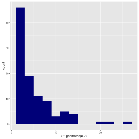
The Geometric Distribution

The geometric distribution is not a stochastic process per se, but it can be represented by one. If we repeatedly flip a coin and then count the number of flips until the first head, and then consider the probability distribution over that count, voilà. That’s the geometric distribution. You might see a head right away, or you might be infinitely unlucky and never see a head. So the distribution is supported over the entirety of the natural numbers.

For illustration, we can encode the coin flipping process in a straightforward recursive manner:

simpleGeometric :: Double -> Terminating Int
simpleGeometric p = loop 1 where
  loop n = do
    accept <- bernoulli p
    if   accept
    then dirac n
    else loop (n + 1)

We start flipping Bernoulli-distributed coins, and if we observe a head we stop and return the number of coins flipped thus far. Otherwise we keep flipping.

The underlying probabilistic phenomena here are the Bernoulli draw, which determines if we’ll terminate, and the dependent Dirac return, which will wrap a terminating value in a point mass. The recursive procedure itself has the pattern of:

• If some condition is met, abort the recursion and return a value.
• Otherwise, keep recursing.

This pattern describes an apomorphism, and the recursion-schemes type signature of ‘apo’ is:

apo :: Corecursive t => (a -> Base t (Either t a)) -> a -> t

It takes a coalgebra that returns an ‘Either’ value wrapped up in a base functor, and uses that coalgebra to drive the recursion. A ‘Left’-returned value halts the recursion, while a ‘Right’-returned value keeps it going.

Don’t be put off by the type of the coalgebra if you’re unfamiliar with apomorphisms - its bark is worse than its bite. Check out my older post on apomorphisms for a brief introduction to them.

With reference to the ‘apo’ type signature, The main thing to choose here is the recursive type that we’ll use to wrap up the ‘ModelF’ base functor. ‘Fix’ might be conceivably simpler to start, so I’ll begin with that. The coalgebra defining the model looks like this:

geoCoalg p n = BernoulliF p (\accept ->
  if   accept
  then Left (Fix (DiracF n))
  else Right (n + 1))

Then given the coalgebra, we can just wrap it up in ‘apo’ to represent the geometric distribution.

geometric :: Double -> Terminating Int
geometric p = free (apo (geoCoalg p) 1)

Since the geometric distribution (weakly) terminates, the program has return type ‘Terminating Int’.

Since we’ve encoded the coalgebra using ‘Fix’, we have to explicitly convert to ‘Free’ via the ‘free’ utility function I defined in the preamble. Recent versions of recursion-schemes have added a ‘Corecursive’ instance for ‘Free’, though, so the superior alternative is to just use that:

geometric :: Double -> Terminating Int
geometric p = apo coalg 1 where
  coalg n = TF.Free (BernoulliF p (\accept ->
    if   accept
    then Left (dirac n)
    else Right (n + 1)))

The point of all this is that we can isolate the core probabilistic phenomena of the recursive process by factoring it out into a coalgebra. The recursion itself takes the form of an apomorphism, which knows nothing about probability or flipping coins or what have you - it just knows how to recurse, or stop.

For illustration, here’s a histogram of samples drawn from the geometric via:

> replicateM 100 (sample (rvar (geometric 0.2)))

An Autoregressive Process

Autoregressive (AR) processes simply use a previous epoch’s output as the current epoch’s input; the number of previous epochs used as input on any given epoch is called the order of the process. An AR(1) process looks like this, for example:

Here \(\epsilon_t\) are independent and identically-distributed random variables that follow some error distribution. In other words, in this model the value \(\alpha + \beta y_{t - 1}\) follows some probability distribution given the last epoch’s output \(y_{t - 1}\) and some parameters \(\alpha\) and \(\beta\).

An autoregressive process doesn’t have any notion of termination built into it, so the purest way to represent one is via an anamorphism. We’ll focus on AR(1) processes in this example:

ar1 :: Double -> Double -> Double -> Double -> Model Double
ar1 a b s = ana coalg where
  coalg x = TF.Free (GaussianF (affine a b x) s (affine a b))

Each epoch is just a Gaussian-distributed affine transformation of the previous epochs’s output. But the problem with using an anamorphism here is that it will just shoot off to infinity, recursing endlessly. This doesn’t do us a ton of good if we want to actually observe the process, so if we want to do that we’ll need to bake in our own conditions for termination. Again we’ll rely on an apomorphism for this; we can just specify how many periods we want to observe the process for, and stop recursing as soon as we exceed that.

There are two ways to do this. We can either get a view of the process at \(n\) periods in the future, or we can get a view of the process over \(n\) periods in the future. I’ll write both, for illustration. The coalgebra for the first is simpler, and looks like:

arCoalg (n, x) = TF.Free (GaussianF (affine a b x) s (\y ->
    if   n <= 0
    then Left (dirac x)
    else Right (pred m, y)))

The coalgebra is saying:

• Given \(x\), let \(z\) have a Gaussian distribution with mean \(\alpha + \beta x\) and standard deviation \(s\).
• If we’re on the last epoch, return \(x\) as a Dirac point mass.
• Otherwise, continue recursing with \(z\) as input to the next epoch.

Now, to observe the process over the next \(n\) periods we can just collect the observations we’ve seen so far in a list. An implementation of the process, apomorphism and all, looks like this:

ar :: Int -> Double -> Double -> Double -> Double -> Terminating [Double]
ar n a b s origin = apo coalg (n, [origin]) where
  coalg (epochs, history@(x:_)) =
    TF.Free (GaussianF (affine a b x) s (\y ->
      if   epochs <= 0
      then Left (dirac (reverse history))
      else Right (pred epochs, y:history)))

(Note that I’m deliberately not handling the error condition here so as to focus on the essence of the coalgebra.)

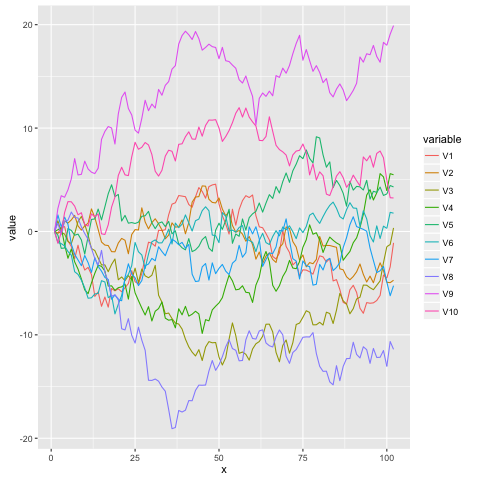
We can generate some traces for it in the standard way. Here’s how we’d sample a 100-long trace from an AR(1) process originating at 0 with \(\alpha = 0\), \(\beta = 1\), and \(s = 1\):

> sample (rvar (ar 100 0 1 1 0))

and here’s a visualization of 10 of those traces:

The Stick-Breaking Process

The stick breaking process is one of any number of whimsical stochastic processes used as prior distributions in nonparametric Bayesian models. The idea here is that we want to take a stick and endlessly break it into smaller and smaller pieces. Every time we break a stick, we recursively take the rest of the stick and break it again, ad infinitum.

Again, if we wanted to represent this endless process very faithfully, we’d use an anamorphism to drive it. But in practice we’re going to only want to break a stick some finite number of times, so we’ll follow the same pattern as the AR process and use an apomorphism to do that:

sbp :: Int -> Double -> Terminating [Double]
sbp n a = apo coalg (n, 1, []) where
  coalg (epochs, stick, sticks) = TF.Free (BetaF 1 a (\p ->
    if   epochs <= 0
    then Left (dirac (reverse (stick : sticks)))
    else Right (pred epochs, (1 - p) * stick, (p * stick):sticks)))

The coalgebra that defines the process says the following:

• Let the location \(p\) of the break on the next (normalized) stick be beta\((1, \alpha)\)-distributed.
• If we’re on the last epoch, return all the pieces of the stick that we broke as a Dirac point mass.
• Otherwise, break the stick again and recurse.

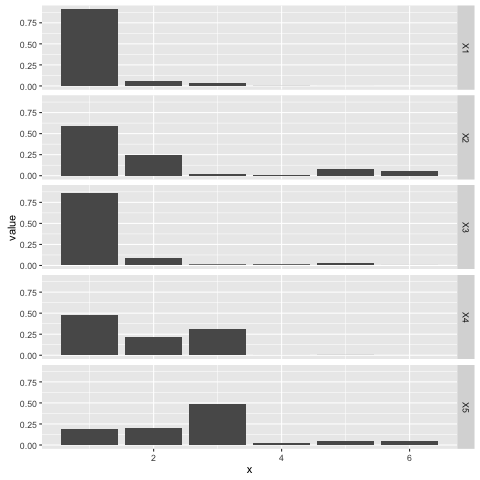
Here’s a plot of five separate draws from a stick breaking process with \(\alpha = 0.2\), each one observed for five breaks. Note that each draw encodes a categorical distribution over the set \(\{1, \ldots, 6\}\); the stick breaking process is a ‘distribution over distributions’ in that sense:

The stick breaking process is useful for developing mixture models with an unknown number of components, for example. The \(\alpha\) parameter can be tweaked to concentrate or disperse probability mass as needed.

Conclusion

This seems like enough for now. I’d be interested in exploring other models generated by recursive processes just to see how they can be encoded, exactly. Basically all of Bayesian nonparametrics is based on using recursive processses as prior distributions, so the Dirichlet process, Chinese Restaurant Process, Indian Buffet Process, etc. should work beautifully in this setting.

Fun fact: back in 2011 before neural networks deep learning had taken over machine learning, Bayesian nonparametrics was probably the hottest research area in town. I used to joke that I’d create a new prior called the Malaysian Takeaway Process for some esoteric nonparametric model and thus achieve machine learning fame, but never did get around to that.

Addendum

I got a question about how I produce these plots. And the answer is the only sane way when it comes to visualization in Haskell: dump the output to disk and plot it with something else. I use R for most of my interactive/exploratory data science-fiddling, as well as for visualization. Python with matplotlib is obviously a good choice too.

Here’s how I made the autoregressive process plot, for example. First, I just produced the actual samples in GHCi:

> samples <- replicateM 10 (sample (rvar (ar 100 0 1 1 0)))

Then I wrote them to disk:

> let render handle = hPutStrLn handle . filter (`notElem` "[]") . show
> withFile "trace.dat" WriteMode (\handle -> mapM_ (render handle) samples)

The following R script will then get you the plot:

require(ggplot2)
require(reshape2)

raw = read.csv('trace.dat', header = F)

d = data.frame(t(raw), x = seq_along(raw))
m = melt(d, id.vars = 'x')

ggplot(m, aes(x, value, colour = variable)) + geom_line()

I used ggplot2 for the other plots as well; check out the ggplot2 functions geom_histogram, geom_bar, and facet_grid in particular.